Chapter 4 Working with tabular data in R (gapminder)
Learning Objectives
- Load external data from a .csv file into a data frame in R with
read_csv()- Find basic properties of a data frames including size, class or type of the columns, names of rows and columns by using
str(),glimpse(),nrow(),ncol(),dim(),length(),colnames(),rownames()- Use
head()andtail()to inspect rows of a data frame.- Generate summary statistics for a data frame
- Use indexing to select rows and columns
- Use logical conditions to select rows and columns
- Add columns and rows to a data frame
- Use
df$new_col <- new_colto add a new column to a data frame.- Use
cbind()to add a new column to a data frame.- Use
rbind()to add a new row to a data frame.- Use
na.omit()to remove rows from a data frame withNAvalues.
Data frames are the de facto data structure for tabular data in R, and what we use for data processing, statistics, and plotting.
A data frame is the representation of data in the format of a table where the columns are vectors that all have the same length. Data frames are analogous to the more familiar spreadsheet in programs such as Excel, with one key difference. Because columns are vectors, each column must contain a single type of data (e.g., characters, integers, factors). For example, here is a figure depicting a data frame comprising a numeric, a character, and a logical vector.
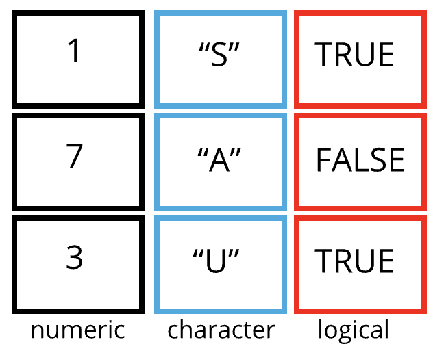
Figure 4.1: Structure of a data frame
As we have seen above, data frames can be created by hand, but most commonly they are generated by the functions like read.csv(), read_csv() or read_table() and others. These functions essentially import the tables or spreadsheets from your hard drive (or the web). We will now demonstrate how to import tabular data using read_csv().
4.1 Importing tabular data
You are going to load the data in R’s memory using the function read_csv() from the readr package, which is part of the tidyverse. You can learn more about the tidyverse collection of packages (here)[https://www.tidyverse.org/]. readr is installed as part as the tidyverse installation. When you load the tidyverse (library(tidyverse)), the core packages (the packages used in most data analyses) are loaded, including readr.
So lets make sure you have the tidyverse packages are installed and loaded.
If you haven’t done so already run the installation of tidyverse like this:
Then load tidyverse into memory like this:
You may have noticed that when you loaded the tidyverse package that you received the following message:
── Conflicts ─────────────────────────────────────── tidyverse_conflicts() ──
✖ dplyr::filter() masks stats::filter()
✖ dplyr::lag() masks stats::lag()
ℹ Use the conflicted package to force all conflicts to become errors
This presents a good opportunity to talk about conflicts. Certain packages we load can end up introducing function names that are already in use by pre-loaded R packages. For instance, when we load the tidyverse package below, we will introduce two conflicting functions: filter() and lag(). This happens because filter and lag are already functions used by the stats package (already pre-loaded in R). What will happen now is that if we, for example, call the filter() function, R will use the dplyr::filter() version and not the stats::filter() one. This happens because, if conflicted, by default R uses the function from the most recently loaded package. Conflicted functions may cause you some trouble in the future, so it is important that we are aware of them so that we can properly handle them, if we want.
To do so, we can use the following functions from the conflicted package:
conflicted::conflict_scout(): Shows us any conflicted functions.conflict_prefer("function", "package_prefered"): Allows us to choose the default function we want from now on.
It is also important to know that we can, at any time, just call the function directly from the package we want, such as stats::filter().
Ok. With that out of the way you are now ready to load the data.
We will use a dataset from gapminder.org containing population information for many countries through time. This is file in CSV format. What is a CSV file?
There are several options how you can access this file:
- Download the gapminder data from this link to a csv file.
Download the file (right mouse click on the link above -> “Save link as” / “Save file as”, or click on the link and after the page loads, press Ctrl+S or choose File -> “Save page as”)
Make sure it’s saved under the name gapminder_data.csv
Save or move the file in the data/ folder within your project.
- Files can also be downloaded directly from the Internet into a local folder of your choice onto your computer using the
download.filefunction in R. The read_csv function can then be executed to read the downloaded file from the download location, for example:
download.file("https://raw.githubusercontent.com/swcarpentry/r-novice-gapminder/main/episodes/data/gapminder_data.csv", destfile = "data/gapminder_data.csv")
gapminder <- read_csv("data/gapminder_data.csv")- Alternatively, you can also read in files directly into R from the Internet by replacing the file paths with a web address in
read_csv. One should note that in doing this no local copy of the csv file is first saved onto your computer. For example:
gapminder <- read_csv("https://raw.githubusercontent.com/swcarpentry/r-novice-gapminder/main/episodes/data/gapminder_data.csv")If you were to type in the code above, it is likely that the read.csv() (note the dot!) function appears in the automatically populated list of functions. This function is different from the read_csv() (note the underscore!) function. read.csv() (with dot) is included in the “base” R packages that come pre-installed with R. Overall, read.csv() behaves similar to read_csv(), with a few notable differences. First, read.csv() coerces column names with spaces and/or special characters to different names (e.g. interview date becomes interview.date). Second, read.csv() stores data as a data.frame, where read_csv() stores data as a tibble. We prefer tibbles because they have nice printing properties among other desirable qualities. Read more about tibbles here.
The second statement in the code above creates a data frame but doesn’t output any data because, as you might recall, assignments (<-) don’t display anything. (Note, however, that read_csv may show informational text about the data frame that is created.)
So let’s check out the data! We can type the name of the object gapminder:
#> # A tibble: 1,704 × 6
#>    country      year      pop continent lifeExp gdpPercap
#>    <chr>       <dbl>    <dbl> <chr>       <dbl>     <dbl>
#>  1 Afghanistan  1952  8425333 Asia         28.8      779.
#>  2 Afghanistan  1957  9240934 Asia         30.3      821.
#>  3 Afghanistan  1962 10267083 Asia         32.0      853.
#>  4 Afghanistan  1967 11537966 Asia         34.0      836.
#>  5 Afghanistan  1972 13079460 Asia         36.1      740.
#>  6 Afghanistan  1977 14880372 Asia         38.4      786.
#>  7 Afghanistan  1982 12881816 Asia         39.9      978.
#>  8 Afghanistan  1987 13867957 Asia         40.8      852.
#>  9 Afghanistan  1992 16317921 Asia         41.7      649.
#> 10 Afghanistan  1997 22227415 Asia         41.8      635.
#> # ℹ 1,694 more rows
read_csv() assumes that fields are delimited by commas. For other delimiters (like semicolon or tab) check out the help: ?read_csv
Note that read_csv() loads the data as a so called “tibble”. A tibble is an extended form of R data frames (as an object of multiple classes tbl_df, tbl, and data.frame). This may sound confusing, but it is really not anything you typically need to deal with when working the data. In fact, it makes it a little more convenient.
As you may recall, a data frame in R is a special case of a list, and a representation of data where the columns are vectors that all have the same length. Because the columns are vectors, they all contain the same type of data (e.g., characters, integers, factors, etc.).
In this tibble you can see the type of data included in each column listed in an abbreviated fashion right below the column names. For instance, the country column is is of type character <chr>, the year is in <dbl> is are floating point number (abbreviated <dbl> for the word ‘double’).
4.2 Inspecting data frames
When calling a tbl_dfobject (like gapminder here), there is already a lot of information about our data frame being displayed such as the number of rows, the number of columns, the names of the columns, and as we just saw the class of data stored in each column. However, there are additional functions to extract this information from data frames. Here is a non-exhaustive list of some of these functions. Let’s try them out!
We already saw how the functions head() and str() can be useful to check the
content and the structure of a data frame. Here is a non-exhaustive list of
functions to get a sense of the content/structure of the data. Let’s try them out!
(Note: most of these functions are “generic”, they can be used on other types of objects besides data frames or tibbles.)
- Summary:
str(gapminder)- structure of the object and information about the class, length and content of each columnsummary(gapminder)- summary statistics for each columnglimpse(gapminder)- returns the number of columns and rows of the tibble, the names and class of each column, and previews as many values will fit on the screen. Unlike the other inspecting functions listed above,glimpse()is not a ‘base R’ function so you need to have thedplyrortibblepackages loaded to be able to execute it.
- Size:
dim(gapminder)- returns a vector with the number of rows in the first element, and the number of columns as the second element (the dimensions of the object)nrow(gapminder)- returns the number of rowsncol(gapminder)- returns the number of columnslength(gapminder)- returns number of columns
- Content:
head(gapminder)- shows the first 6 rowstail(gapminder)- shows the last 6 rows
- Names:
names(gapminder)- returns the column names (synonym ofcolnames()fordata.frameobjects)rownames(gapminder)- returns the row names
Challenge
Based on the output of
str(gapminder), can you answer the following questions?
- What is the class of the object
gapminder?- How many rows and how many columns are in this object?
- How many counties have been recorded in this dataset?
4.3 Indexing and subsetting data frames
Our gapminder data frame has rows and columns (it has 2 dimensions), if we want to extract some specific data from it, we need to specify the “coordinates” (i.e., indices) we want from it. Row numbers come first, followed by column numbers.
## first element in the first column of the tibble
gapminder[1, 1]
## first element in the 5th column of the tibble
gapminder[1, 5]
## first column of the tibble
gapminder[1]
## first column of the tibble (as a vector)
gapminder[[1]]

## the 3rd row of the tibble
gapminder[3, ]
## first three elements in the 6th column of the tibble
gapminder[1:3, 6]
## equivalent to head(gapminder)
gapminder[1:6, ]

## Excludig with '-'
## The whole tibble, except the first column
gapminder[, -1]
## equivalent to head(gapminder)
gapminder[-c(6:nrow(gapminder)),]
Subsetting a tibble with [ always results in a tibble. However, note that different ways of specifying these coordinates lead to results with different classes. Below are some example for data.frame objects.
gapminder_df <- as.data.frame(gapminder)
gapminder_df[1, 1]   # first element in the first column of the data frame (as a vector)
gapminder_df[, 1]    # first column in the data frame (as a vector)
gapminder_df[1]      # first column in the data frame (as a data.frame)
An alternative to subsetting tibbles (and data frames) is to calling their column names directly.
gapminder["country"]       # Result is a tibble
gapminder[, "country"]     # Result is a tibble
gapminder[["country"]]     # Result is a vector
gapminder$country          # Result is a vector
RStudio knows about the columns in your data frame, so you can take advantage of the autocompletion feature to get the full and correct column name.
Challenge
Create a
tibble(gapminder_200) containing only the observations from row 200 of thegapminderdataset.Notice how
nrow()gave you the number of rows in atibble?
- Use that number to pull out just that last row in the data frame.
- Compare that with what you see as the last row using
tail()to make sure it’s meeting expectations.- Pull out that last row using
nrow()instead of the row number.- Create a new data frame object (
gapminder_last) from that last row.Use
nrow()to extract the row that is in the middle of the data frame. Store the content of this row in an object namedgapminder_middle.Combine
nrow()with the-notation above to reproduce the behavior ofhead(gapminder)keeping just the first through 6th rows of the gapminder dataset.
4.4 Conditional subsetting
A very common need when working with tables is the need to extract a subset of a data frame based on certain conditions, depending on the actual content of the table. For example, we may want to look only at the data from Oceania. In this case we can use logical conditions, exactly like we did above with vector subsetting. In base R this can be done like this:
# the condition:
# returns a logical vector of the length of the column
gapminder$continent == "Oceania"

# use this vector to extract rows and all columns
# note the comma: we want *all* columns
gapminder[gapminder$continent == "Oceania", ]

# assign extract to a new data frame
gapminder_oceania <- gapminder[gapminder$continent == "Oceania", ]
This is also a possibility (but slower):
gapminder_oceania <- subset(gapminder, continent == "Oceania")
nrow(gapminder_oceania) # 24 records for Oceania
#> [1] 24Challenge
From the
gapminderdata create a new table namedgap_seAsia_1990with the following countries:
“Myanmar”,“Thailand”,“Cambodia”,“Vietnam”,“Laos” and from the year 1990 only.
These commands are from the R base package. We will discuss a different (and more readable!) method of subsetting using functions from the tidyverse package later on.
4.5 Adding and removing rows and columns
There are three major ways to add columns to a table:
- Add a new column with new values.
- Add a new column with values derived from one or more existing columns in the table.
- Combine (or ‘join’) two tables based on a common unique record identifier.
Here we will look at with the first one: add a new column with new values.
To add a new column to the data frame we can use the cbind() function There also is a bind_cols() function from dplyr package (part of the tidyverse). An important difference with bind_cols() is that it displays an error message when you try to combine with vector that has fewer or more elements than the number of rows in the table. cbind() on the other hand, silently repeats values or rows, so you might introduce errors and be unaware of it.
id_column <- 1:nrow(gapminder) # create a unique ID number for each row
gapminder_with_id <- cbind(gapminder, id_column)
glimpse(gapminder_with_id)
#> Rows: 1,704
#> Columns: 7
#> $ country <chr> "Afghanistan", "Afghanistan", "Afghanistan", "Afghanistan", …
#> $ year <dbl> 1952, 1957, 1962, 1967, 1972, 1977, 1982, 1987, 1992, 1997, …
#> $ pop <dbl> 8425333, 9240934, 10267083, 11537966, 13079460, 14880372, 12…
#> $ continent <chr> "Asia", "Asia", "Asia", "Asia", "Asia", "Asia", "Asia", "Asi…
#> $ lifeExp <dbl> 28.801, 30.332, 31.997, 34.020, 36.088, 38.438, 39.854, 40.8…
#> $ gdpPercap <dbl> 779.4453, 820.8530, 853.1007, 836.1971, 739.9811, 786.1134, …
#> $ id_column <int> 1, 2, 3, 4, 5, 6, 7, 8, 9, 10, 11, 12, 13, 14, 15, 16, 17, 1…Alternatively, we can also add a new column adding the new column name after the $ sign then assigning the value, like below. Note that this will change the original data frame, which you may not always want to do.
gapminder$row_numbers <- c(1:nrow(gapminder))
gapminder$all_false <- FALSE  # what do you think will happen here?
There is an equivalent function to cbind(), rbind() to add a new row to a data frame. I use this far less frequently than the column equivalent. The one thing to keep in mind is that the row to be added to the data frame needs to match the order and type of columns in the data frame. Remember that R’s way to store multiple different data types in one object is a list. So if we wanted to add a new row to gapminder we would say:
new_row <- data.frame(country="Greece", year=2017,
                pop=12345, continent = "Europe", lifeExp = 30.3,
                gdpPercap = 1000)

gapminder_withnewrow <- rbind(gapminder, new_row)
tail(gapminder_withnewrow)
#> # A tibble: 6 × 6
#> country year pop continent lifeExp gdpPercap
#> <chr> <dbl> <dbl> <chr> <dbl> <dbl>
#> 1 Zimbabwe 1987 9216418 Africa 62.4 706.
#> 2 Zimbabwe 1992 10704340 Africa 60.4 693.
#> 3 Zimbabwe 1997 11404948 Africa 46.8 792.
#> 4 Zimbabwe 2002 11926563 Africa 40.0 672.
#> 5 Zimbabwe 2007 12311143 Africa 43.5 470.
#> 6 Greece 2017 12345 Europe 30.3 1000Equivalently there is a bind_rows function available in tidyverse. One of the main reasons for using bind_rows over rbind is to combine two data frames having different number of columns. rbind throws an error in such a case whereas bind_rows assigns “NA” to those rows of columns missing in one of the data frames where the value is not provided by the data frames. Here is a systematic review of differences between the two.
There is also add_row fro the tibble package which allows you to specify where to insert the row. You can find out more with ?add_row.
A convenient function to know about is na.omit(). It will remove all rows from a data frame that have at least one column with NA values. The function drop_na() from tidyverse works similarly and lets you name specific columns with NA.
Challenge
- Given the following data frame:
What would you expect the following commands to return?