Chapter 3 Domain specific graphs
Learning Objectives
- Be aware of specialized graph packages and know where to look for them
- Understand the basic structure of iheatmapr, tmap, and visNetwork examples
- Modify parameters of provided graph examples
ggplot can get you a long way, but if you need to do a particular, more complex graph it is worth checking if there might be an R package for that. Typically it would do one type of visualization and do that really well. Below are a few examples.
3.1 Heatmaps (e.g. iheatmapr)
The iheatmapr package specializes in creating interactive heatmaps, that range from standard heatmaps to relatively complex ones, that can be built up iteratively. It uses the plotly for interactivity.
The example below is taken from https://ropensci.github.io/iheatmapr/index.html.
The data mapped are from a matrix that contains the yearly number of measles cases from 1930-2001 for US states.
library(iheatmapr)
data(measles, package = "iheatmapr")

main_heatmap(measles, name = "Measles<br>Cases", x_categorical = FALSE,
             layout = list(font = list(size = 8))) %>%
  add_col_groups(ifelse(1930:2001 < 1961,"No","Yes"),
                  side = "bottom", name = "Vaccine<br>Introduced?",
                  title = "Vaccine?",
                  colors = c("lightgray","blue")) %>%
  add_col_labels(ticktext = seq(1930,2000,10),font = list(size = 8)) %>%
  add_row_labels(size = 0.3,font = list(size = 6)) %>%
  add_col_summary(layout = list(title = "Average<br>across<br>states"),
                  yname = "summary")  %>%
  add_col_title("Measles Cases from 1930 to 2001", side= "top") %>%
  add_row_summary(groups = TRUE,
                  type = "bar",
                  layout = list(title = "Average<br>per<br>year",
                                font = list(size = 8)))
Note that iheatmapr has a Bioconductor dependency, so if you receive a message package ‘S4Vectors’ is not available do this:
if (!requireNamespace("BiocManager", quietly = TRUE))
    install.packages("BiocManager")

BiocManager::install("S4Vectors")3.2 Networks (e.g. visNetwork)
visNetwork is an R interface to the ‘vis.js’ JavaScript library, a package to visualize networks in an interactive fashion. It takes a table of nodes (vertices) and a table of edges (links) as inputs. The example below is taken from Katherine Ognyanova’s tutorial and represents a network of hyperlinks and mentions among various news sources.
library('visNetwork')
nodes <- read.csv("https://github.com/cengel/R-data-viz/raw/master/demo-data/network/Dataset1-Media-Example-NODES.csv", header=T, as.is=T)
links <- read.csv("https://github.com/cengel/R-data-viz/raw/master/demo-data/network/Dataset1-Media-Example-EDGES.csv", header=T, as.is=T)
nodes$shape <- "dot"
nodes$shadow <- TRUE # Nodes will drop shadow
nodes$title <- nodes$media # Text on click
nodes$label <- nodes$type.label # Node label
nodes$size <- nodes$audience.size # Node size
nodes$borderWidth <- 2 # Node border width

nodes$color.background <- c("slategrey", "tomato", "gold")[nodes$media.type]
nodes$color.border <- "black"
nodes$color.highlight.background <- "orange"
nodes$color.highlight.border <- "darkred"

visNetwork(nodes, links) %>%
  visOptions(highlightNearest = TRUE,
             selectedBy = "type.label")
3.3 Maps (e.g. tmap)
The tmap package is designed to visualize spatial data distributions in geographic space, so called “thematic maps”. The example is adapted from mtennekes and shows a map of crimes registered during October 2015. We combine several layers, one with the outline of London, one with the river Thames, and one with the actual crime densities.
For this demo we first need to download the data. If you have your working directory set to R-data-viz and it contains a folder called data, this will download and extract the map data into a subfolder of your data folder, called map:
download.file("https://github.com/cengel/R-data-viz/raw/master/demo-data/map.zip",
              "data/map.zip")
unzip("data/map.zip", exdir="data")
Now, here is the map.
#> Warning in tm_style_gray(title = "Crimes in Greater London\nOctober
#> 2015"): tm_style_gray is deprecated as of tmap version 2.0. Please use
#> tm_style("gray", ...) instead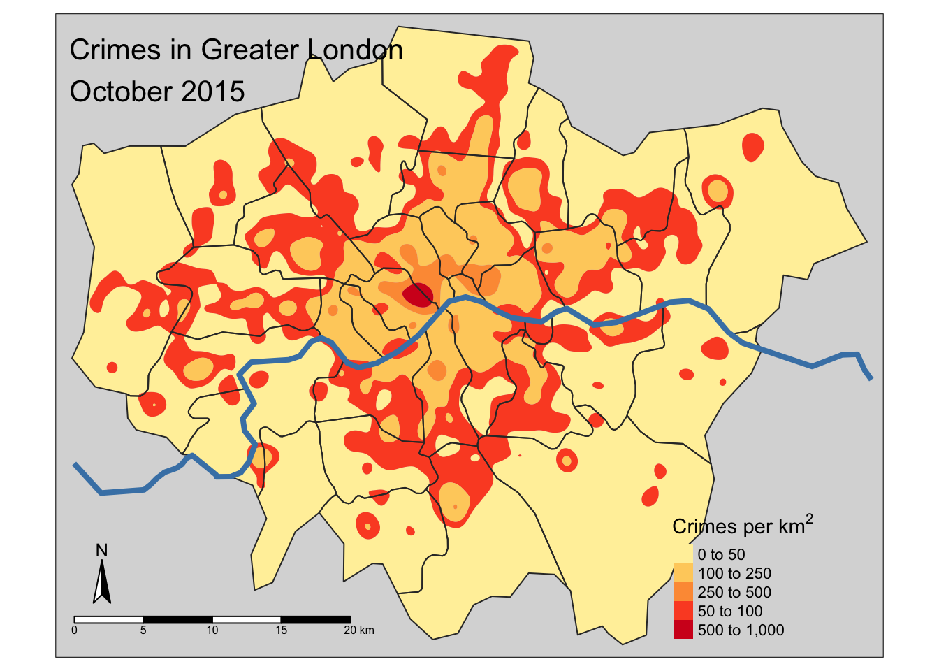
library(tmap)
library(tmaptools)
suppressPackageStartupMessages(library(sf))

london <- st_read("data/map", "London", quiet = TRUE)
crime_densities <- st_read("data/map", "Crimes", quiet = TRUE)
thames <- st_read("data/map", "Thames", quiet = TRUE)

tm_shape(crime_densities) +
  tm_fill(col = "level", palette = "YlOrRd",
    title = expression("Crimes per " * km^2)) +
tm_shape(london) + tm_borders() +
tm_shape(thames) + tm_lines(col = "steelblue", lwd = 4) +
tm_compass(position = c("left", "bottom")) +
tm_scale_bar(position = c("left", "bottom")) +
tm_style_gray(title = "Crimes in Greater London\nOctober 2015")
Good starting places to look for additional examples and packages are the R Graph Gallery: https://www.r-graph-gallery.com/all-graphs/ and the CRAN Task View: https://CRAN.R-project.org/view=Graphics.