Chapter 1 Data Manipulation using dplyr
Learning Objectives
- Select columns in a data frame with the
dplyrfunctionselect.- Select rows in a data frame according to filtering conditions with the
dplyrfunctionfilter.- Direct the output of one
dplyrfunction to the input of another function with the ‘pipe’ operator%>%.- Add new columns to a data frame that are functions of existing columns with
mutate.- Understand the split-apply-combine concept for data analysis.
- Use
summarize,group_by, andcountto split a data frame into groups of observations, apply a summary statistics for each group, and then combine the results.- Join two tables by a common variable.
Manipulation of data frames is a common task when you start exploring your data in R and dplyr is a package for making tabular data manipulation easier.
Brief recap: Packages in R are sets of additional functions that let you do more stuff. Functions like
str()ordata.frame(), come built into R; packages give you access to more of them. Before you use a package for the first time you need to install it on your machine, and then you should import it in every subsequent R session when you need it.
If you haven’t, please install the tidyverse package.
tidyverse is an “umbrella-package” that installs a series of packages useful for data analysis which work together well. Some of them are considered core packages (among them tidyr, dplyr, ggplot2), because you are likely to use them in almost every analysis. Other packages, like lubridate (to work wiht dates) or haven (for SPSS, Stata, and SAS data) that you are likely to use not for every analysis are also installed.
If you type the following command, it will load the core tidyverse packages.
If you need to use functions from tidyverse packages other than the core packages, you will need to load them separately.
1.1 What is dplyr?
dplyr is one part of a larger tidyverse that enables you to work
with data in tidy data formats. “Tidy datasets are easy to manipulate, model and visualise, and have a specific structure: each variable is a column, each observation is a row, and each type of observational unit is a table.” (From Wickham, H. (2014): Tidy Data https://www.jstatsoft.org/article/view/v059i10)
The package dplyr provides convenient tools for the most common data manipulation tasks. It is built to work directly with data frames, which is one of the most common data formats to work with.
To learn more about dplyr after the workshop, you may want to check out the handy data transformation with dplyr cheatsheet.
Let’s begin with loading our sample data into a data frame.
We will be working a small subset of the data from the Stanford Open Policing Project. It contains information about traffic stops in the state of Mississippi during January 2013 to mid-July of 2016.
#> # A tibble: 211,211 × 11
#>    id         stop_date  county_name county_fips police_department driver_gender
#>    <chr>      <date>     <chr>             <dbl> <chr>             <chr>
#>  1 MS-2013-0… 2013-01-01 Jones             28067 Mississippi High… male
#>  2 MS-2013-0… 2013-01-01 Lauderdale        28075 Mississippi High… male
#>  3 MS-2013-0… 2013-01-01 Pike              28113 Mississippi High… male
#>  4 MS-2013-0… 2013-01-01 Hancock           28045 Mississippi High… male
#>  5 MS-2013-0… 2013-01-01 Holmes            28051 Mississippi High… male
#>  6 MS-2013-0… 2013-01-01 Jackson           28059 Mississippi High… female
#>  7 MS-2013-0… 2013-01-01 Jackson           28059 Mississippi High… female
#>  8 MS-2013-0… 2013-01-01 Grenada           28043 Mississippi High… female
#>  9 MS-2013-0… 2013-01-01 Holmes            28051 Mississippi High… male
#> 10 MS-2013-0… 2013-01-01 Holmes            28051 Mississippi High… male
#> # ℹ 211,201 more rows
#> # ℹ 5 more variables: driver_birthdate <date>, driver_race <chr>,
#> #   officer_id <chr>, driver_age <dbl>, violation <chr>
You may have noticed that by using read_csv we have generated an object
of class tbl_df, also known as a “tibble”. Tibble’s data
structure is very similar to a data frame. For our purposes the relevant differences
are that
- it tries to recognize and
datetypes
- it tries to recognize and
- the output displays the data type of each column under its name, and
- it only prints the first few rows of data and only as many columns as
fit on one screen. If we wanted to print all columns we can use the print command, and set the
widthparameter toInf. To print the first 6 rows for example we would do this:print(my_tibble, n=6, width=Inf).
- it only prints the first few rows of data and only as many columns as
fit on one screen. If we wanted to print all columns we can use the print command, and set the
We are going to learn some of the most common dplyr functions:
select(): subset columnsfilter(): subset rows on conditionsmutate(): create new columns by using information from other columnsgroup_by()andsummarize(): create summary statistics on grouped dataarrange(): sort resultscount(): count discrete values
1.2 Selecting columns and filtering rows
To select columns of a data frame with dplyr, use select(). The first argument to this function is the data frame (stops), and the subsequent arguments are the columns to keep. You may have done something similar in the past using subsetting. select() is essentially doing the same thing as subsetting, using a package (dplyr) instead of R’s base functions.
select(stops, county_name, driver_gender, driver_birthdate, driver_race)

# this is the same as subsetting in base R:
stops[c("county_name", "driver_gender", "driver_birthdate","driver_race")]
Alternatively, if you are selecting columns adjacent to each other, you can use a : to select a range of columns, read as “select columns from ___ to ___.”
#> # A tibble: 211,211 × 4
#>    county_name driver_gender driver_birthdate driver_race
#>    <chr>       <chr>         <date>           <chr>
#>  1 Jones       male          1950-06-14       Black
#>  2 Lauderdale  male          1967-04-06       Black
#>  3 Pike        male          1974-04-15       Black
#>  4 Hancock     male          1981-03-23       White
#>  5 Holmes      male          1992-08-03       White
#>  6 Jackson     female        1960-05-02       White
#>  7 Jackson     female        1953-03-16       White
#>  8 Grenada     female        1993-06-14       White
#>  9 Holmes      male          1947-12-11       White
#> 10 Holmes      male          1984-07-14       White
#> # ℹ 211,201 more rows
It is worth knowing that dplyr is backed by another package with a number of helper functions, which provide convenient functions to select columns based on their names. For example:
#> # A tibble: 211,211 × 4
#>    driver_gender driver_birthdate driver_race driver_age
#>    <chr>         <date>           <chr>            <dbl>
#>  1 male          1950-06-14       Black               63
#>  2 male          1967-04-06       Black               46
#>  3 male          1974-04-15       Black               39
#>  4 male          1981-03-23       White               32
#>  5 male          1992-08-03       White               20
#>  6 female        1960-05-02       White               53
#>  7 female        1953-03-16       White               60
#>  8 female        1993-06-14       White               20
#>  9 male          1947-12-11       White               65
#> 10 male          1984-07-14       White               28
#> # ℹ 211,201 more rows
Other examles are: ends_with(), contains(), last_col() and more. Check out the tidyselect reference for more.
To choose rows based on specific criteria, we can use the filter() function. The argument after the dataframe is the condition we want our resulting data frame to adhere to.
#> # A tibble: 3,528 × 11
#>    id         stop_date  county_name county_fips police_department driver_gender
#>    <chr>      <date>     <chr>             <dbl> <chr>             <chr>
#>  1 MS-2013-0… 2013-01-02 Yazoo             28163 Mississippi High… male
#>  2 MS-2013-0… 2013-01-02 Yazoo             28163 Mississippi High… female
#>  3 MS-2013-0… 2013-01-02 Yazoo             28163 Mississippi High… male
#>  4 MS-2013-0… 2013-01-02 Yazoo             28163 Mississippi High… female
#>  5 MS-2013-0… 2013-01-02 Yazoo             28163 Mississippi High… male
#>  6 MS-2013-0… 2013-01-03 Yazoo             28163 Mississippi High… male
#>  7 MS-2013-0… 2013-01-03 Yazoo             28163 Mississippi High… male
#>  8 MS-2013-0… 2013-01-04 Yazoo             28163 Mississippi High… male
#>  9 MS-2013-0… 2013-01-04 Yazoo             28163 Mississippi High… male
#> 10 MS-2013-0… 2013-01-04 Yazoo             28163 Mississippi High… female
#> # ℹ 3,518 more rows
#> # ℹ 5 more variables: driver_birthdate <date>, driver_race <chr>,
#> #   officer_id <chr>, driver_age <dbl>, violation <chr>
We can also specify multiple conditions within the filter() function. We can combine conditions using either “and” or “or” statements. In an “and” statement, an observation (row) must meet all conditions in order to be included in the resulting dataframe. To form “and” statements within dplyr, we can pass our desired conditions as arguments in the filter() function, separated by commas:
#> # A tibble: 4 × 11
#>   id          stop_date  county_name county_fips police_department driver_gender
#>   <chr>       <date>     <chr>             <dbl> <chr>             <chr>
#> 1 MS-2013-33… 2013-06-18 Yazoo             28163 Mississippi High… male
#> 2 MS-2014-36… 2014-07-31 Yazoo             28163 Mississippi High… female
#> 3 MS-2015-01… 2015-01-10 Yazoo             28163 Mississippi High… male
#> 4 MS-2015-50… 2015-10-16 Yazoo             28163 Mississippi High… female
#> # ℹ 5 more variables: driver_birthdate <date>, driver_race <chr>,
#> #   officer_id <chr>, driver_age <dbl>, violation <chr>
We can also form “and” statements with the & operator instead of commas:
#> # A tibble: 4 × 11
#>   id          stop_date  county_name county_fips police_department driver_gender
#>   <chr>       <date>     <chr>             <dbl> <chr>             <chr>
#> 1 MS-2013-33… 2013-06-18 Yazoo             28163 Mississippi High… male
#> 2 MS-2014-36… 2014-07-31 Yazoo             28163 Mississippi High… female
#> 3 MS-2015-01… 2015-01-10 Yazoo             28163 Mississippi High… male
#> 4 MS-2015-50… 2015-10-16 Yazoo             28163 Mississippi High… female
#> # ℹ 5 more variables: driver_birthdate <date>, driver_race <chr>,
#> #   officer_id <chr>, driver_age <dbl>, violation <chr>
In an “or” statement, observations must meet at least one of the specified conditions. To form “or” statements we use the logical operator for “or”, which is the vertical bar (|):
#> # A tibble: 4,470 × 11
#>    id         stop_date  county_name county_fips police_department driver_gender
#>    <chr>      <date>     <chr>             <dbl> <chr>             <chr>
#>  1 MS-2013-0… 2013-01-02 Yazoo             28163 Mississippi High… male
#>  2 MS-2013-0… 2013-01-02 Yazoo             28163 Mississippi High… female
#>  3 MS-2013-0… 2013-01-02 Yazoo             28163 Mississippi High… male
#>  4 MS-2013-0… 2013-01-02 Yazoo             28163 Mississippi High… female
#>  5 MS-2013-0… 2013-01-02 Yazoo             28163 Mississippi High… male
#>  6 MS-2013-0… 2013-01-03 Yazoo             28163 Mississippi High… male
#>  7 MS-2013-0… 2013-01-03 Yazoo             28163 Mississippi High… male
#>  8 MS-2013-0… 2013-01-04 Yazoo             28163 Mississippi High… male
#>  9 MS-2013-0… 2013-01-04 Yazoo             28163 Mississippi High… male
#> 10 MS-2013-0… 2013-01-04 Yazoo             28163 Mississippi High… female
#> # ℹ 4,460 more rows
#> # ℹ 5 more variables: driver_birthdate <date>, driver_race <chr>,
#> #   officer_id <chr>, driver_age <dbl>, violation <chr>
Here are some other ways to subset rows:
- by row number:
slice(stops, 1:3) # rows 1-3 - rows with highest or lowest values of a variable:
slice_min(stops, driver_age) # likewise slice_max()
- random rows:
slice_sample(stops, n = 5) # number of rows to selectslice_sample(stops, prop = .0001) # fraction of rows to select
To sort rows by variables use the arrange() function:
#> # A tibble: 211,211 × 11
#>    id         stop_date  county_name county_fips police_department driver_gender
#>    <chr>      <date>     <chr>             <dbl> <chr>             <chr>
#>  1 MS-2013-0… 2013-02-09 Adams             28001 Mississippi High… male
#>  2 MS-2013-1… 2013-03-02 Adams             28001 Mississippi High… female
#>  3 MS-2013-1… 2013-03-16 Adams             28001 Mississippi High… female
#>  4 MS-2013-1… 2013-03-20 Adams             28001 Mississippi High… female
#>  5 MS-2013-1… 2013-04-06 Adams             28001 Mississippi High… female
#>  6 MS-2013-2… 2013-04-13 Adams             28001 Mississippi High… female
#>  7 MS-2013-2… 2013-04-19 Adams             28001 Mississippi High… female
#>  8 MS-2013-2… 2013-04-21 Adams             28001 Mississippi High… female
#>  9 MS-2013-2… 2013-04-24 Adams             28001 Mississippi High… male
#> 10 MS-2013-2… 2013-04-24 Adams             28001 Mississippi High… male
#> # ℹ 211,201 more rows
#> # ℹ 5 more variables: driver_birthdate <date>, driver_race <chr>,
#> #   officer_id <chr>, driver_age <dbl>, violation <chr>
1.3 Pipes
What if you wanted to filter and select on the same data? For example, lets find drivers over 85 years and only keep the violation and gender columns. There are three ways to do this: use intermediate steps, nested functions, or pipes.
- Intermediate steps:
With intermediate steps, you create a temporary data frame and use that as input to the next function.
This is readable, but can clutter up your workspace with lots of objects that you have to name individually. With multiple steps, that can be hard to keep track of.
- Nested functions
You can also nest functions (i.e. place one function inside of another).
This is handy, but can be difficult to read if too many functions are nested as things are evaluated from the inside out (in this case, filtering, then selecting).
- Pipes!
The last option, called “pipes”. Pipes let you take the output of one function and send it directly to the next, which is useful when you need to do many things to the same dataset.
There are now two Pipes in R:
%>%(called magrittr pipe; made available via themagrittrpackage, installed automatically withdplyr) or|>(called native R pipe and it comes preinstalled with R v4.1.0 onwards).
Both the pipes, by and large, function similarly with a few differences (For more information, check: https://www.tidyverse.org/blog/2023/04/base-vs-magrittr-pipe/). The choice of which pipe to be used can be changed in the Global settings in R studio and once that is done, you can type the pipe with: Ctrl + Shift + M if you have a PC or Cmd + Shift + M if you have a Mac.
The following example is run using the magrittr pipe, which I will use for the rest of the tutorial.
However, the output will be same with the native pipe so you can feel free to use this pipe as well.
In the above, we use the pipe to send the stops data first through
filter() to keep rows where driver_race is Black, then through select()
to keep only the officer_id and stop_date columns. Since %>% takes
the object on its left and passes it as the first argument to the function on
its right, we don’t need to explicitly include it as an argument to the
filter() and select() functions anymore.
If we wanted to create a new object with this smaller version of the data, we could do so by assigning it a new name:
senior_drivers <- stops %>%
  filter(driver_age > 85) %>%
  select(violation, driver_gender, driver_race)

senior_drivers
#> # A tibble: 3 × 3
#> violation driver_gender driver_race
#> <chr> <chr> <chr>
#> 1 Seat belt male White
#> 2 Speeding male White
#> 3 Seat belt male BlackNote that the final data frame is the leftmost part of this expression.
Some may find it helpful to read the pipe like the word “then”. For instance, in the above example, we take the dataframe stops, then we filter for rows with driver_age > 85, then we select columns violation, driver_gender and driver_race. The dplyr functions by themselves are somewhat simple, but by combining them into linear workflows with the pipe, we can accomplish more complex data wrangling operations.
Challenge
Using pipes, subset the
stopsdata to include stops in Tunica county only and retain the columnsstop_date,driver_age, andviolation. Bonus: sort the table by driver age.
1.4 Add new columns
Frequently you’ll want to create new columns based on the values in existing columns or. For this we’ll use mutate(). We can also reassign values to an existing column with that function.
Be aware that new and edited columns will not permanently be added to the existing data frame, munless we explicitly save the output.
So here is an example using the year() function (from the lubridate package, which is part of the tidyverse) to extract the year of the drivers’ birth:
We can keep adding columns like this, for example, the decade of the birth year:
We are beginning to see the power of piping. Here is a slightly expanded example, where we select the column birth_cohort that we have created and send it to plot:
stops %>%
  mutate(birth_year = year(driver_birthdate),
         birth_cohort = floor(birth_year/10)*10,
         birth_cohort = factor(birth_cohort)) %>%
    select(birth_cohort) %>%
    plot()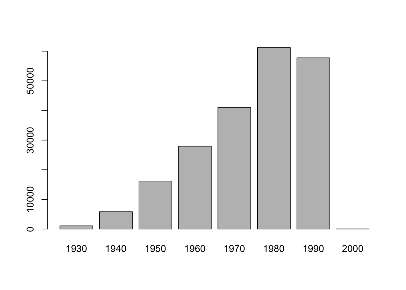
Figure 1.1: Driver Birth Cohorts
Mutate can also be used in conjunction with logical conditions. For example, we could create a new column, where we assign everyone born after the year 2000 to a group “millenial” and everyone before to “pre-millenial”.
In order to do this we take advantage of the ifelse function:
ifelse(a_logical_condition, if_true_return_this, if_false_return_this)
In conjunction with mutate, this works like this:
stops %>%
  mutate(cohort = ifelse(year(driver_birthdate) < 2000, "pre-millenial", "millenial")) %>%
  select(driver_birthdate, cohort)
#> # A tibble: 211,211 × 2
#> driver_birthdate cohort
#> <date> <chr>
#> 1 1950-06-14 pre-millenial
#> 2 1967-04-06 pre-millenial
#> 3 1974-04-15 pre-millenial
#> 4 1981-03-23 pre-millenial
#> 5 1992-08-03 pre-millenial
#> 6 1960-05-02 pre-millenial
#> 7 1953-03-16 pre-millenial
#> 8 1993-06-14 pre-millenial
#> 9 1947-12-11 pre-millenial
#> 10 1984-07-14 pre-millenial
#> # ℹ 211,201 more rowsMore advanced conditional recoding can be done with case_when().
Challenge
Create a new data frame from the
stopsdata that meets the following criteria: contains only theviolationcolumn for female drivers of age 50 that were stopped on a Sunday. For this add a new column to your data frame calledweekday_of_stopcontaining the number of the weekday when the stop occurred. Use thewday()function fromlubridate(Sunday = 1).Think about how the commands should be ordered to produce this data frame!
1.5 What is split-apply-combine?
Many data analysis tasks can be approached using the split-apply-combine paradigm:
- split the data into groups,
- apply some analysis to each group, and
- combine the results.
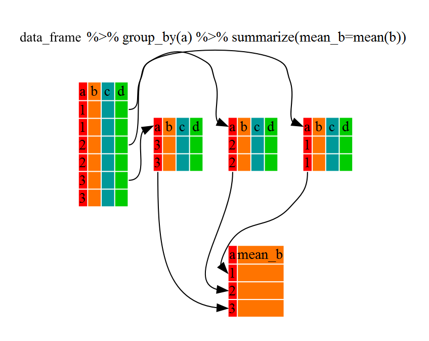
Figure 1.2: Split - Apply - Combine
dplyr makes this possible through the use of the group_by() function.
group_by() is often used together with summarize(), which collapses each
group into a single-row summary of that group. group_by() takes as arguments
the column names that contain the categorical variables for which you want
to calculate the summary statistics. So to view the mean age for black and white drivers:
stops %>%
  group_by(driver_race) %>% # needs a dategorical variable to group by
  summarize(mean_age = mean(driver_age, na.rm=TRUE))
#> # A tibble: 3 × 2
#> driver_race mean_age
#> <chr> <dbl>
#> 1 Black 34.2
#> 2 White 36.2
#> 3 <NA> 34.5If we wanted to remove the line where driver_race is NA we could insert a filter() in the chain:
stops %>%
  filter(!is.na(driver_race)) %>%
  group_by(driver_race) %>%
  summarize(mean_age = mean(driver_age, na.rm=TRUE))
#> # A tibble: 2 × 2
#> driver_race mean_age
#> <chr> <dbl>
#> 1 Black 34.2
#> 2 White 36.2Recall that is.na() is a function that determines whether something is an NA. The ! symbol negates the result, so we’re asking for everything that is not an NA.
You can also group by multiple columns:
stops %>%
  filter(!is.na(driver_race)) %>%
  group_by(county_name, driver_race) %>%
  summarize(mean_age = mean(driver_age, na.rm=TRUE))
#> # A tibble: 163 × 3
#> # Groups: county_name [82]
#> county_name driver_race mean_age
#> <chr> <chr> <dbl>
#> 1 Adams Black 36.2
#> 2 Adams White 40.0
#> 3 Alcorn Black 34.6
#> 4 Alcorn White 33.6
#> 5 Amite Black 37.5
#> 6 Amite White 42.1
#> 7 Attala Black 36.4
#> 8 Attala White 38.6
#> 9 Benton Black 34.7
#> 10 Benton White 32.0
#> # ℹ 153 more rowsNote that the output is a “grouped” tibble, grouped by county_name. What it means is that the tibble “remembers” the grouping of the counties, so for any operation you would do after that it will take that grouping into account.
To obtain an “ungrouped” tibble, you can use the ungroup function1:
stops %>%
  filter(!is.na(driver_race)) %>%
  group_by(county_name, driver_race) %>%
  summarize(mean_age = mean(driver_age, na.rm=TRUE)) %>%
  ungroup()
#> # A tibble: 163 × 3
#> county_name driver_race mean_age
#> <chr> <chr> <dbl>
#> 1 Adams Black 36.2
#> 2 Adams White 40.0
#> 3 Alcorn Black 34.6
#> 4 Alcorn White 33.6
#> 5 Amite Black 37.5
#> 6 Amite White 42.1
#> 7 Attala Black 36.4
#> 8 Attala White 38.6
#> 9 Benton Black 34.7
#> 10 Benton White 32.0
#> # ℹ 153 more rowsOnce the data are grouped, you can also summarize multiple variables at the same time (and not necessarily on the same variable). For instance, we could add a column indicating the standard deviation for the age in each group:
stops %>%
  filter(!is.na(driver_race)) %>%
  group_by(county_name, driver_race) %>%
  summarize(mean_age = mean(driver_age, na.rm=TRUE),
            sd_age = sd(driver_age, na.rm=TRUE))
#> # A tibble: 163 × 4
#> # Groups: county_name [82]
#> county_name driver_race mean_age sd_age
#> <chr> <chr> <dbl> <dbl>
#> 1 Adams Black 36.2 14.9
#> 2 Adams White 40.0 15.8
#> 3 Alcorn Black 34.6 12.9
#> 4 Alcorn White 33.6 13.6
#> 5 Amite Black 37.5 13.4
#> 6 Amite White 42.1 14.9
#> 7 Attala Black 36.4 13.8
#> 8 Attala White 38.6 15.5
#> 9 Benton Black 34.7 12.0
#> 10 Benton White 32.0 9.50
#> # ℹ 153 more rowsIt is sometimes useful to rearrange the result of a query to inspect the values. For that we use arrange(). To sort in descending order, we need to add the desc() function. For instance, we can sort on mean_age to put the groups with the highest mean age first:
stops %>%
  filter(!is.na(driver_race)) %>%
  group_by(county_name, driver_race) %>%
  summarize(mean_age = mean(driver_age, na.rm=TRUE),
            sd_age = sd(driver_age, na.rm=TRUE)) %>%
  arrange(desc(mean_age))
#> # A tibble: 163 × 4
#> # Groups: county_name [82]
#> county_name driver_race mean_age sd_age
#> <chr> <chr> <dbl> <dbl>
#> 1 Amite White 42.1 14.9
#> 2 Quitman White 42.0 16.6
#> 3 Sharkey White 41.1 14.2
#> 4 Coahoma White 40.7 15.7
#> 5 Warren White 40.5 15.1
#> 6 Claiborne White 40.5 15.4
#> 7 Issaquena White 40.4 13.7
#> 8 Yazoo White 40.3 15.1
#> 9 Adams White 40.0 15.8
#> 10 Smith Black 39.9 14.5
#> # ℹ 153 more rows1.6 Tallying
When working with data, it is also common to want to know the number of
observations found for categorical variables. For this, dplyr
provides count(). For example, if we wanted to see how many traffic stops each officer recorded:
Bu default, count will name the column with the counts n. We can change this by explicitly providing a value for the name argument:
We can optionally sort the results in descending order by adding sort=TRUE:
count() calls group_by() transparently before counting the total number of records for each category.
These are equivalent alternatives to the above:
stops %>%
  group_by(officer_id) %>%
  summarize(n_stops = n()) %>% # n() returns the group size
  arrange(desc(n_stops))

stops %>%
  group_by(officer_id) %>%
  tally(sort = TRUE, name = "n_stops") # tally() requires group_by before counting
We can also count subgroups within groups:
Challenge
Which 5 counties were the ones with the most stops in 2013? Hint: use the year() function from lubridate.
1.7 Joining two tables
It is not uncommon that we have our data spread out in different tables and need to bring those together for analysis. In this example we will combine the numbers of stops for black and white drivers per county together with the numbers of the black and white total population for these counties. The population data are the estimated values of the 5 year average from the 2011-2015 American Community Survey (ACS):
#> # A tibble: 82 × 5
#>    County      FIPS black_pop white_pop bw_pop
#>    <chr>      <dbl>     <dbl>     <dbl>  <dbl>
#>  1 Jones      28067     19711     47154  66865
#>  2 Lauderdale 28075     33893     43482  77375
#>  3 Pike       28113     21028     18282  39310
#>  4 Hancock    28045      4172     39686  43858
#>  5 Holmes     28051     15498      3105  18603
#>  6 Jackson    28059     30704    101686 132390
#>  7 Grenada    28043      9417     11991  21408
#>  8 Scott      28123     10562     16920  27482
#>  9 Wayne      28153      8015     12154  20169
#> 10 Bolivar    28011     21648     11197  32845
#> # ℹ 72 more rows
In a first step we count all the stops per county.
#> # A tibble: 82 × 2
#>    county_name n_stops
#>    <chr>         <int>
#>  1 Adams           942
#>  2 Alcorn         3345
#>  3 Amite          2921
#>  4 Attala         4203
#>  5 Benton          214
#>  6 Bolivar        4526
#>  7 Calhoun        1658
#>  8 Carroll        1788
#>  9 Chickasaw      3869
#> 10 Choctaw         613
#> # ℹ 72 more rows
We will then pipe this into our next operation where we bring the two tables together. We will use left_join, which returns all rows from the left table, and all columns from the left and the right table. As ID, which uniquely identifies the corresponding records in each table we use the County names.
#> # A tibble: 82 × 6
#>    county_name n_stops  FIPS black_pop white_pop bw_pop
#>    <chr>         <int> <dbl>     <dbl>     <dbl>  <dbl>
#>  1 Adams           942 28001     17757     12856  30613
#>  2 Alcorn         3345 28003      4281     31563  35844
#>  3 Amite          2921 28005      5416      7395  12811
#>  4 Attala         4203 28007      8194     10649  18843
#>  5 Benton          214 28009      3078      5166   8244
#>  6 Bolivar        4526 28011     21648     11197  32845
#>  7 Calhoun        1658 28013      3991     10103  14094
#>  8 Carroll        1788 28015      3470      6702  10172
#>  9 Chickasaw      3869 28017      7549      9522  17071
#> 10 Choctaw         613 28019      2596      5661   8257
#> # ℹ 72 more rows
Now we can, for example calculate the stop rate, i.e. the number of stops per population in each county.
Challenge
Which county has the highest and which one the lowest stop rate? Use the snippet from above and pipe into the additional operations to do this.
dplyr join functions are generally equivalent to merge from the R base install, but there are a few advantages.
For all the possible joins see ?dplyr::join
There are currently some experimental features implemented for the
summaryfunction tthat might change how grouping and ungrouping are handled in the future↩︎