Chapter 2 Data Manipulation using tidyr
Learning Objectives
- Understand the concept of a wide and a long table format and for which purpose those formats are useful.
- Understand what key-value pairs are.
- Reshape a data frame from long to wide format and back with the
pivot_widerandpivot_longercommands from thetidyrpackage.- Export a data frame to a .csv file.
dplyr pairs well with tidyr which enables you to flexibly convert between different tabular formats for plotting and analysis.
The package tidyr addresses a very common problem of needing to reshape your data for plotting, for statistical summaries, or for use by different R functions.
2.1 About long and wide table format
The “long” format is where:
- each column is a variable
- each row is an observation
- each value must have its own cell
In a “wide” format we see modifications to rule 1, where each column no longer represents a single variable. Instead, columns can represent different levels or values of the same variable. Each observation type has its own column, like surveys, where each row could be an interview respondent and each column represents one possible answer to the same question. Another example are repeated observations over time, where each column represents, for example, a year.
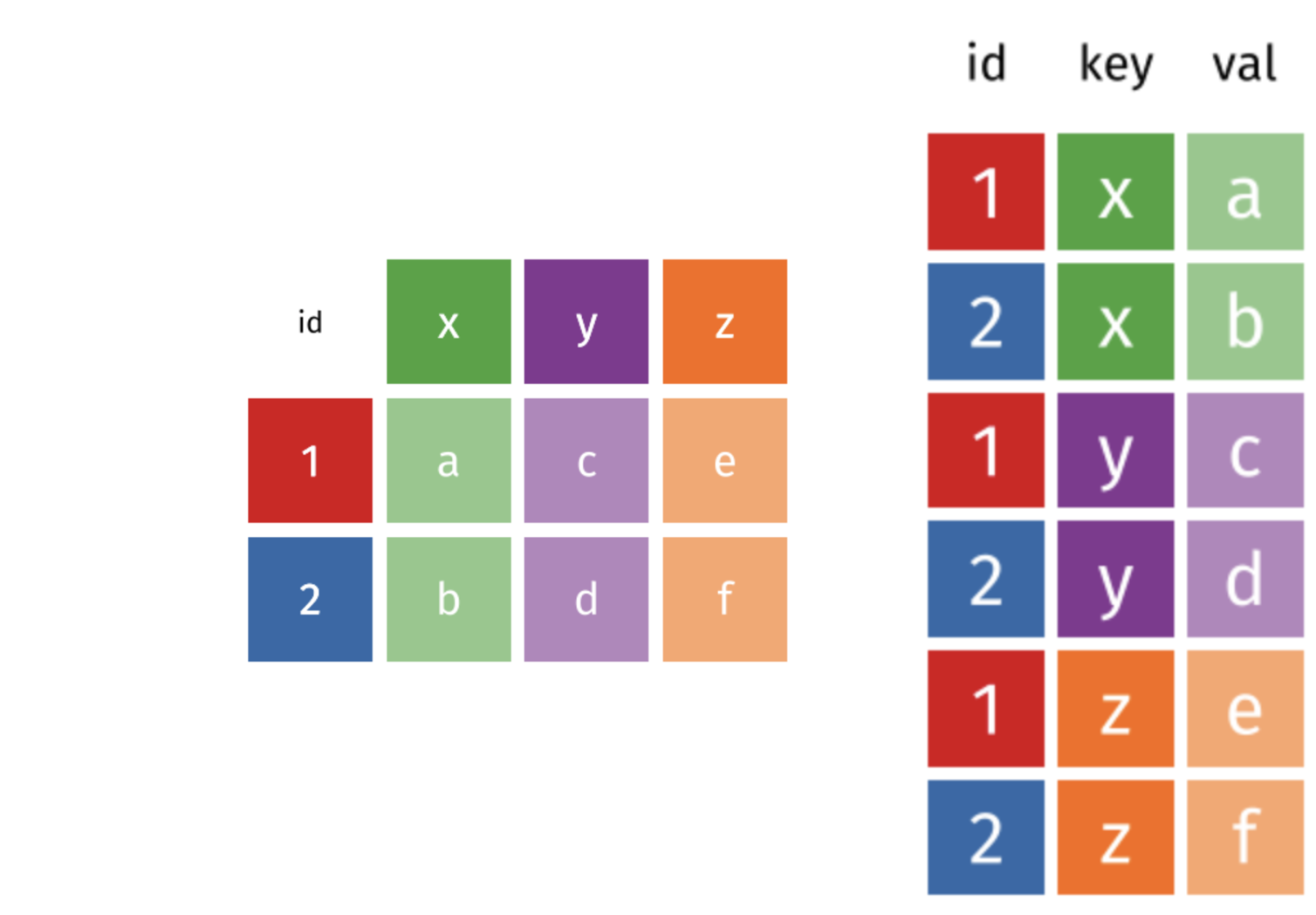
Figure 2.1: Wide (left) vs. Long (right) Table Format
Long and wide data frame layouts affect readability. You may find that visually you may prefer the “wide” format, since you can see more of the data on the screen. However, all of the R functions we have used thus far expect for your data to be in a “long” data format. It simplifies the use of the functions and makes your code clearer and more efficient. The long format is more machine readable and is closer to the formatting of databases.
Moving back and forth between these formats can be cumbersome, and tidyr provides the tools for this to make it easier.
To learn more about tidyr after the workshop, you may want to check out this cheatsheet about tidyr.
Challenge 1
Is stops in a long or wide format?
2.2 Long to Wide with pivot_wider
Now let’s see this in action. First, using dplyr, let’s create a data frame with the counts of different violations for each county:
#>   county_name                violation n_violations
#> 1       Adams        Breaks-Lights-etc            7
#> 2       Adams         Careless driving           48
#> 3       Adams License-Permit-Insurance          118
#> 4       Adams         Other or unknown           35
#> 5       Adams                Seat belt          229
#> 6       Adams                 Speeding          505
Now, to make this long data wide, we use pivot_wider from tidyr to turn the different violation types into columns, where each possible value of the violation variable receives its own column.
pivot_wider() takes three principal arguments:
- the data
- the
names_fromcolumn variable whose values will become new column names. - the
values_fromcolumn variable whose values will fill the new column cells.
We’ll use a pipe into pivot_wider so we can leave out the data argument.
violations_wide <- violations %>%
  pivot_wider(names_from = violation,
              values_from = n_violations)

violations_wide
#> # A tibble: 82 × 7
#> county_name `Breaks-Lights-etc` `Careless driving` `License-Permit-Insurance`
#> <chr> <int> <int> <int>
#> 1 Adams 7 48 118
#> 2 Alcorn 62 100 737
#> 3 Amite 47 86 370
#> 4 Attala 99 113 526
#> 5 Benton 3 9 73
#> 6 Bolivar 57 139 1034
#> 7 Calhoun 26 38 383
#> 8 Carroll 26 40 323
#> 9 Chickasaw 42 53 1378
#> 10 Choctaw 8 6 73
#> # ℹ 72 more rows
#> # ℹ 3 more variables: `Other or unknown` <int>, `Seat belt` <int>,
#> # Speeding <int>It is worth taking a look at ?pivot_wider. The function takes many more arguments which can help in reshaping, renaming the new columns, and instructions for how to treat the values or how to fill missing values.
2.3 Wide to long with pivot_longer
What if we had the opposite problem, and wanted to go from a wide to long
format? For that, we use pivot_longer, which will increase the number of rows and decrease the number of columns.
We are gathering the multiple violation columns and turn them into a pair of new variables. One variable includes the column names as values, and the other variable contains the values in each cell previously associated with the column names.
pivot_longer() takes four principal arguments:
- the data
colsare the names of the columns we use to fill the a new values variable (or to drop).- the
names_toa string specifying the name of the column to create from the data stored in the column names (cols) - the
values_towhich is also a string, specifying the name of the column to create from the data stored in cell values.
So, to go backwards from violations_wide, and exclude county_name from the long format, we would do the following:
violations_long <- violations_wide %>%
  pivot_longer(cols = -county_name,        # exclude column with county name
               names_to = "violation",     # name is a string!
               values_to = "n_violations")            # also a string

violations_long
#> # A tibble: 492 × 3
#> county_name violation n_violations
#> <chr> <chr> <int>
#> 1 Adams Breaks-Lights-etc 7
#> 2 Adams Careless driving 48
#> 3 Adams License-Permit-Insurance 118
#> 4 Adams Other or unknown 35
#> 5 Adams Seat belt 229
#> 6 Adams Speeding 505
#> 7 Alcorn Breaks-Lights-etc 62
#> 8 Alcorn Careless driving 100
#> 9 Alcorn License-Permit-Insurance 737
#> 10 Alcorn Other or unknown 418
#> # ℹ 482 more rowsWe could also have used a specification for what columns to include. This can be
useful if you have a large number of identifying columns, and it’s easier to
specify what to gather than what to leave alone. And if the columns are adjacent to each other, we don’t even need to list them all out – we can use the : operator!
violations_wide %>%
  pivot_longer(cols = `Breaks-Lights-etc`:Speeding,      # this also works
               names_to = "violation",
               values_to = "n")
#> # A tibble: 492 × 3
#> county_name violation n
#> <chr> <chr> <int>
#> 1 Adams Breaks-Lights-etc 7
#> 2 Adams Careless driving 48
#> 3 Adams License-Permit-Insurance 118
#> 4 Adams Other or unknown 35
#> 5 Adams Seat belt 229
#> 6 Adams Speeding 505
#> 7 Alcorn Breaks-Lights-etc 62
#> 8 Alcorn Careless driving 100
#> 9 Alcorn License-Permit-Insurance 737
#> 10 Alcorn Other or unknown 418
#> # ℹ 482 more rowsThere are many powerful operations you can do with the pivot_* functions. To learn more review the vignette:
Challenge
1.From the stops dataframe create a wide data frame
tr_widewith “year” as columns, each row is a different violation, and the values are the number of traffic stops per each violation, roughly like this:
violation | 2013 | 2014 | 2015 ...Break-Lights | 65 | 54| 67 ...Speeding | 713 | 948| 978 ......Use
year()from the lubridate package. Hint: You will need to summarize and count the traffic stops before reshaping the table.
- Now take the data frame, and make it long again, so each row is a unique violation - year combination, like this:
violation | year | n of stopsSpeeding | 2013 | 65Speeding | 2014 | 54... etc
2.4 Exporting data
Similar to the read_csv() function used for reading CSV files into R, there is a write_csv() function that generates CSV files from data frames.
Before using write_csv(), we are going to create a new folder, data_output,
in our working directory that will store this generated dataset. We don’t want
to write generated datasets in the same directory as our raw data. It’s good
practice to keep them separate. The data folder should only contain the raw,
unaltered data, and should be left alone to make sure we don’t delete or modify
it. In contrast, our script will generate the contents of the data_output
directory, so even if the files it contains are deleted, we can always
re-generate them.
We can now save the table generated above in our data_output
folder: