Chapter 1 Introduction to spatial data in R

Learning Objectives

  • Read table with geo coordinates into sf object
  • Read shapefiles into sf object
  • Examine sf objects
  • Use base plot with sf objects and attribute data
  • Read GeoTiff single and multiband into a SpatRaster object
  • Examine SpatRaster objects

1.1 The sf package

The sf1 package was first released on CRAN in late October 2016, and has in the mean time superseded the original R Package for storing and manipulating spatial data, sp, which was first released in 2005. sp is still actively maintained, but less often used now, so you should be aware of it, but we will not teach it here.

Cumulative downloads of sf and sp from CRAN

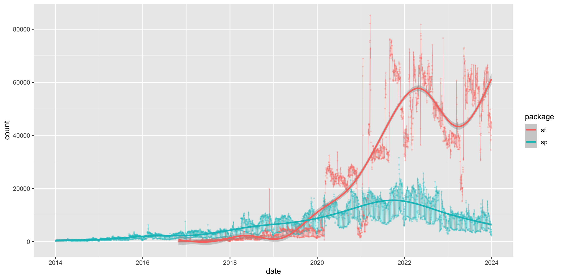
Figure 1.1: Cumulative downloads of sf and sp from CRAN

sf implements a formal standard called “Simple Features” that specifies a storage and access model of spatial geometries (point, line, polygon). A feature geometry is called simple when it consists of points connected by straight line pieces, and does not intersect itself. This standard has been adopted widely, not only by spatial databases such as PostGIS, but also more recent standards such as GeoJSON.

If you work with PostGis or GeoJSON you may have come across the WKT (well-known text) format (Fig 1.1 and 1.2)

Well-Known-Text Geometry primitives  (wikipedia)

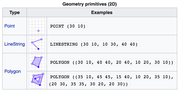
Figure 1.2: Well-Known-Text Geometry primitives (wikipedia)

Well-Known-Text Multipart geometries (wikipedia)

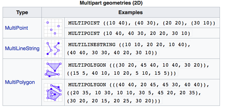
Figure 1.3: Well-Known-Text Multipart geometries (wikipedia)

sf implements this standard natively in R. In sf spatial objects are stored as a tabular format (data frame) with a special column that contains the information for the geometry coordinates. That special column holds a list with the same length as the number of rows in the data frame. Each of the individual list elements then can be of any length needed to hold the coordinates that correspond to an individual feature.

sf objects are built up using the following structures:

  1. sfg - simple feature geometry (one feature)
  2. sfc - simple feature collection (a collection of sfg)
  3. sf - simple feature object (sfc with data attributes)

So to create a spatial sf object manually the basic steps would be:

I. Create geometric objects (topology)

Geometric objects (simple features) can be created from a numeric vector, matrix or a list with the coordinates. They are called sfg objects for Simple Feature Geometry.b There are functions that help create simple feature geometries, like st_point(), st_linestring(), st_polygon() and more.

II. Combine all individual single feature objects for the special column.

The feature geometries are then combined into a Simple Feature Collection with st_sfc(). which is nothing other than a simple feature geometry list-column. The sfc object also holds the bounding box and the projection information.

III. Add attributes.

Lastly, we add the attributes to the the simple feature collection with the st_sf() function. This function extends the well known data frame in R with a column that holds the simple feature collection.

To create a network of highways we would first generate LINESTRINGs as simple feature geometries out of a matrix with coordinates:

lnstr_sfg1 <- st_linestring(matrix(runif(6), ncol=2)) 
lnstr_sfg2 <- st_linestring(matrix(runif(6), ncol=2)) 
class(lnstr_sfg1)
#> [1] "XY"         "LINESTRING" "sfg"

We would then combine this into a simple feature collection :

(lnstr_sfc <- st_sfc(lnstr_sfg1, lnstr_sfg2)) 
#> Geometry set for 2 features 
#> Geometry type: LINESTRING
#> Dimension:     XY
#> Bounding box:  xmin: 0.1106804 ymin: 0.2781413 xmax: 0.9729355 ymax: 0.8550861
#> CRS:           NA
#> LINESTRING (0.805963 0.2781413, 0.1711646 0.850...
#> LINESTRING (0.9179095 0.8550861, 0.9729355 0.41...

And lastly create a data frame from above to generate the sf object:

dfr <- data.frame(id = c("hwy1", "hwy2"), 
                  cars_per_hour = c(78, 22))
(lnstr_sf <- st_sf(dfr , lnstr_sfc))
#> Simple feature collection with 2 features and 2 fields
#> Geometry type: LINESTRING
#> Dimension:     XY
#> Bounding box:  xmin: 0.1106804 ymin: 0.2781413 xmax: 0.9729355 ymax: 0.8550861
#> CRS:           NA
#>     id cars_per_hour                      lnstr_sfc
#> 1 hwy1            78 LINESTRING (0.805963 0.2781...
#> 2 hwy2            22 LINESTRING (0.9179095 0.855...

There are many methods available in the sf package, to find out use

methods(class="sf")
#>   [1] [                            [[<-                        
#>   [3] [<-                          $<-                         
#>   [5] aggregate                    anti_join                   
#>   [7] arrange                      as.data.frame               
#>   [9] cbind                        coerce                      
#>  [11] crs                          dbDataType                  
#>  [13] dbWriteTable                 distance                    
#>  [15] distinct                     dplyr_reconstruct           
#>  [17] drop_na                      duplicated                  
#>  [19] ext                          extract                     
#>  [21] filter                       full_join                   
#>  [23] gather                       group_by                    
#>  [25] group_split                  identify                    
#>  [27] initialize                   inner_join                  
#>  [29] left_join                    lines                       
#>  [31] mask                         merge                       
#>  [33] mutate                       nest                        
#>  [35] pivot_longer                 pivot_wider                 
#>  [37] plot                         points                      
#>  [39] polys                        print                       
#>  [41] rasterize                    rbind                       
#>  [43] rename_with                  rename                      
#>  [45] right_join                   rowwise                     
#>  [47] sample_frac                  sample_n                    
#>  [49] select                       semi_join                   
#>  [51] separate_rows                separate                    
#>  [53] show                         slice                       
#>  [55] slotsFromS3                  spread                      
#>  [57] st_agr                       st_agr<-                    
#>  [59] st_area                      st_as_s2                    
#>  [61] st_as_sf                     st_as_sfc                   
#>  [63] st_bbox                      st_boundary                 
#>  [65] st_break_antimeridian        st_buffer                   
#>  [67] st_cast                      st_centroid                 
#>  [69] st_collection_extract        st_concave_hull             
#>  [71] st_convex_hull               st_coordinates              
#>  [73] st_crop                      st_crs                      
#>  [75] st_crs<-                     st_difference               
#>  [77] st_drop_geometry             st_exterior_ring            
#>  [79] st_filter                    st_geometry                 
#>  [81] st_geometry<-                st_inscribed_circle         
#>  [83] st_interpolate_aw            st_intersection             
#>  [85] st_intersects                st_is_full                  
#>  [87] st_is_valid                  st_is                       
#>  [89] st_join                      st_line_merge               
#>  [91] st_m_range                   st_make_valid               
#>  [93] st_minimum_bounding_circle   st_minimum_rotated_rectangle
#>  [95] st_nearest_points            st_node                     
#>  [97] st_normalize                 st_point_on_surface         
#>  [99] st_polygonize                st_precision                
#> [101] st_reverse                   st_sample                   
#> [103] st_segmentize                st_set_precision            
#> [105] st_shift_longitude           st_simplify                 
#> [107] st_snap                      st_sym_difference           
#> [109] st_transform                 st_triangulate_constrained  
#> [111] st_triangulate               st_union                    
#> [113] st_voronoi                   st_wrap_dateline            
#> [115] st_write                     st_z_range                  
#> [117] st_zm                        summarise                   
#> [119] svc                          text                        
#> [121] transform                    transmute                   
#> [123] ungroup                      unite                       
#> [125] unnest                       vect                        
#> see '?methods' for accessing help and source code

Here are some of the other highlights of sf you might be interested in:

  • provides fast I/O, particularly relevant for large files
  • spatial functions that rely on GEOS and GDAL and PROJ external libraries are directly linked into the package, so no need to load additional external packages (like in sp)
  • sf objects can be plotted directly with ggplot
  • sf directly reads from and writes to spatial databases such as PostGIS
  • sf is compatible with the tidyvderse approach, (but see some pitfalls here)

Note that sp and sf are not the only way spatial objects are conceptualized in R. Other spatial packages may use their own class definitions for spatial data (for example spatstat).

There are packages specifically for the GeoJSON and for that reason are more lightweight, for example geojson

Usually you can find functions that convert objects to and from these formats.

Challenge

Generate an sf point object.

  1. Create a matrix pts of random numbers with two columns and as many rows as you like. These are your points.
  2. Create a dataframe attrib_df with the same number of rows as your pts matrix and a column that holds an attribute. You can make up any attribute.
  3. Use the appropriate commands and pts an sf object with a gemoetry column of class sfc_POINT.
  4. Try to subset your spatial object using the attribute you have added and the way you are used to from regular data frames.
  5. How do you determine the bounding box of your spatial object?

1.2 Creating a spatial object from a table with coordinates

Often in your research might have a spreadsheet that contains latitude, longitude and perhaps some attribute values. You know how to read the spreadsheet into a tabular format (tibble) with dplyr::read_table or dplyr::read_csv. We can then very easily convert the table into a spatial object in R.

An sf object can be created from a data frame in the following way. We take advantage of the st_as_sf() function which converts foreign objects into an sf object. Similarly to above, it requires an argument coords, which in the case of point data needs to be a vector that specifies the data frame’s columns for the longitude and latitude (x,y) coordinates.

my_sf_object <- st_as_sf(myDataframe, coords)

st_as_sf() creates a new object and leaves the original data frame untouched.

We use read_csv() to read philly_homicides.csv into a tibble in R and name it homicides_df.

homicides_df <- read_csv("data/philly_homicides.csv")
#> Rows: 3883 Columns: 10
#> ── Column specification ────────────────────────────────────────────────────────
#> Delimiter: ","
#> chr  (3): SECTOR, LOCATION_BLOCK, TEXT_GENERAL_CODE
#> dbl  (5): DC_DIST, UCR_GENERAL, OBJ_ID, POINT_X, POINT_Y
#> date (1): DISPATCH_DATE
#> time (1): DISPATCH_TIME
#> 
#> ℹ Use `spec()` to retrieve the full column specification for this data.
#> ℹ Specify the column types or set `show_col_types = FALSE` to quiet this message.

We convert the homicides_df data frame into an sf object with st_as_sf()

library(sf)

homicides_sf <- st_as_sf(homicides_df, coords = c("POINT_X", "POINT_Y"))

Now let’s check what we did here. First lets look at the column names:

names(homicides_sf)
#> [1] "DC_DIST"           "SECTOR"            "DISPATCH_DATE"    
#> [4] "DISPATCH_TIME"     "LOCATION_BLOCK"    "UCR_GENERAL"      
#> [7] "OBJ_ID"            "TEXT_GENERAL_CODE" "geometry"

Compare this with the original table:

names(homicides_df)
#>  [1] "DC_DIST"           "SECTOR"            "DISPATCH_DATE"    
#>  [4] "DISPATCH_TIME"     "LOCATION_BLOCK"    "UCR_GENERAL"      
#>  [7] "OBJ_ID"            "TEXT_GENERAL_CODE" "POINT_X"          
#> [10] "POINT_Y"

Note the additional geometry list-column which now holds the simple feature collection with the coordinates of all the points.

The st_geometryfunction provides some helpful details about the spatial geometry of the object we created:

st_geometry(homicides_sf)
#> Geometry set for 3883 features 
#> Geometry type: POINT
#> Dimension:     XY
#> Bounding box:  xmin: -75.26809 ymin: 39.87503 xmax: -74.95874 ymax: 40.13086
#> CRS:           NA
#> First 5 geometries:
#> POINT (-75.1568 39.98804)
#> POINT (-75.17873 39.92801)
#> POINT (-75.18275 39.92607)
#> POINT (-75.18092 39.92704)
#> POINT (-75.17204 39.92463)

And here is what we see when we type the name of the sf object:

homicides_sf
#> Simple feature collection with 3883 features and 8 fields
#> Geometry type: POINT
#> Dimension:     XY
#> Bounding box:  xmin: -75.26809 ymin: 39.87503 xmax: -74.95874 ymax: 40.13086
#> CRS:           NA
#> # A tibble: 3,883 × 9
#>    DC_DIST SECTOR DISPATCH_DATE DISPATCH_TIME LOCATION_BLOCK  UCR_GENERAL OBJ_ID
#>      <dbl> <chr>  <date>        <time>        <chr>                 <dbl>  <dbl>
#>  1      22 1      2014-09-14    16:00         1800 BLOCK W M…         100      1
#>  2       1 B      2006-01-14    00:00         2000 BLOCK MIF…         100      1
#>  3       1 B      2006-04-01    16:05         S 22ND ST /SNY…         100      1
#>  4       1 B      2006-05-10    11:13         2100 BLOCK MC …         100      1
#>  5       1 E      2006-07-01    12:42         2100 BLOCK S H…         100      1
#>  6       1 F      2006-07-09    19:13         1800 BLOCK SNY…         100      1
#>  7       1 B      2006-07-10    23:20         1800 BLOCK S 2…         100      1
#>  8       1 J      2006-07-16    01:26         2200 BLOCK JAC…         100      1
#>  9       1 J      2006-10-03    20:37         2200 BLOCK S H…         100      1
#> 10       1 A      2006-10-16    19:46         1900 BLOCK MC …         100      1
#> # ℹ 3,873 more rows
#> # ℹ 2 more variables: TEXT_GENERAL_CODE <chr>, geometry <POINT>

We now use st_crs() to check on the projection.

st_crs(homicides_sf)
#> Coordinate Reference System: NA

To make it a complete geographical object we use st_crs() to assign the WGS84 projection, which has the EPSG code 4326:

st_crs(homicides_sf) <- 4326
st_crs(homicides_sf)
#> Coordinate Reference System:
#>   User input: EPSG:4326 
#>   wkt:
#> GEOGCRS["WGS 84",
#>     ENSEMBLE["World Geodetic System 1984 ensemble",
#>         MEMBER["World Geodetic System 1984 (Transit)"],
#>         MEMBER["World Geodetic System 1984 (G730)"],
#>         MEMBER["World Geodetic System 1984 (G873)"],
#>         MEMBER["World Geodetic System 1984 (G1150)"],
#>         MEMBER["World Geodetic System 1984 (G1674)"],
#>         MEMBER["World Geodetic System 1984 (G1762)"],
#>         MEMBER["World Geodetic System 1984 (G2139)"],
#>         MEMBER["World Geodetic System 1984 (G2296)"],
#>         ELLIPSOID["WGS 84",6378137,298.257223563,
#>             LENGTHUNIT["metre",1]],
#>         ENSEMBLEACCURACY[2.0]],
#>     PRIMEM["Greenwich",0,
#>         ANGLEUNIT["degree",0.0174532925199433]],
#>     CS[ellipsoidal,2],
#>         AXIS["geodetic latitude (Lat)",north,
#>             ORDER[1],
#>             ANGLEUNIT["degree",0.0174532925199433]],
#>         AXIS["geodetic longitude (Lon)",east,
#>             ORDER[2],
#>             ANGLEUNIT["degree",0.0174532925199433]],
#>     USAGE[
#>         SCOPE["Horizontal component of 3D system."],
#>         AREA["World."],
#>         BBOX[-90,-180,90,180]],
#>     ID["EPSG",4326]]

Wow this is long! It is usually more helpful to just retrieve the proj4string like so:

st_crs(homicides_sf)$proj4string
#> [1] "+proj=longlat +datum=WGS84 +no_defs"

Here we assigned the projection in a separate step. You can also assign it at the same time when you read the csv file in with st_as_sf:

homicides_sf <- st_as_sf(homicides_df, coords = c("POINT_X", "POINT_Y"), 
                         crs = st_crs(4326)) # assign CRS here

We will save this object as a shapefile on our hard drive for later use. (Note that by default st_write checks if the file already exists, and if so it will not overwrite it. If you need to force it to overwrite use the option delete_layer = TRUE.)

st_write(homicides_sf, "data/PhillyHomicides", driver = "ESRI Shapefile")
# to force the save: 
st_write(homicides_sf, "data/PhillyHomicides", driver = "ESRI Shapefile", delete_layer = TRUE)

Challenge

Read in Schools.csv, convert to a spatial sf object and save out as a shapefile. Assume that the coordinates are in WGS84 geographic projection. I should mention that sf works with piping. You may or may not find that convenient.

1.3 Loading shape files into R

sf relies on the powerful GDAL library, which is automatically linked in when loading sf. The GDAL provides the functionality to read and write spatial files of many formats. The command st_drivers() returns the available drivers.

For shape files we can use st_read(), which takes the path of the directory with the shapefile as argument.

# read in
philly_sf <- st_read("data/Philly/")
#> Reading layer `PhillyTotalPopHHinc' from data source 
#>   `/Users/cengel/Anthro/R_Class/R_Workshops/R-spatial/data/Philly' 
#>   using driver `ESRI Shapefile'
#> Simple feature collection with 384 features and 17 fields
#> Geometry type: MULTIPOLYGON
#> Dimension:     XY
#> Bounding box:  xmin: 1739497 ymin: 457343.7 xmax: 1764030 ymax: 490544.9
#> Projected CRS: Albers

Take a look at what we’ve got:

str(philly_sf) 
#> Classes 'sf' and 'data.frame':   384 obs. of  18 variables:
#>  $ STATEFP10 : chr  "42" "42" "42" "42" ...
#>  $ COUNTYFP10: chr  "101" "101" "101" "101" ...
#>  $ TRACTCE10 : chr  "036301" "036400" "036600" "034803" ...
#>  $ GEOID10   : num  4.21e+10 4.21e+10 4.21e+10 4.21e+10 4.21e+10 ...
#>  $ NAME10    : chr  "363.01" "364" "366" "348.03" ...
#>  $ NAMELSAD10: chr  "Census Tract 363.01" "Census Tract 364" "Census Tract 366" "Census Tract 348.03" ...
#>  $ MTFCC10   : chr  "G5020" "G5020" "G5020" "G5020" ...
#>  $ FUNCSTAT10: chr  "S" "S" "S" "S" ...
#>  $ ALAND10   : num  2322732 4501110 1004313 1271533 1016206 ...
#>  $ AWATER10  : num  66075 8014 1426278 8021 0 ...
#>  $ INTPTLAT10: chr  "+40.0895349" "+40.1127747" "+39.9470272" "+40.0619427" ...
#>  $ INTPTLON10: chr  "-074.9667387" "-074.9789137" "-075.1404472" "-075.0023705" ...
#>  $ GISJOIN   : chr  "G4201010036301" "G4201010036400" "G4201010036600" "G4201010034803" ...
#>  $ Shape_area: num  2388806 4509124 2430591 1279556 1016207 ...
#>  $ Shape_len : num  6851 10567 9257 4928 5920 ...
#>  $ medHHinc  : num  54569 NA 130139 56667 69981 ...
#>  $ totalPop  : num  3695 703 1643 4390 3807 ...
#>  $ geometry  :sfc_MULTIPOLYGON of length 384; first list element: List of 1
#>   ..$ :List of 1
#>   .. ..$ : num [1:55, 1:2] 1763647 1763473 1763366 1763378 1763321 ...
#>   ..- attr(*, "class")= chr [1:3] "XY" "MULTIPOLYGON" "sfg"
#>  - attr(*, "sf_column")= chr "geometry"
#>  - attr(*, "agr")= Factor w/ 3 levels "constant","aggregate",..: NA NA NA NA NA NA NA NA NA NA ...
#>   ..- attr(*, "names")= chr [1:17] "STATEFP10" "COUNTYFP10" "TRACTCE10" "GEOID10" ...

Note again the geometry column. Also note the many other values (or attributes) that are included.

Let’s check the geometry column:

st_geometry(philly_sf) 
#> Geometry set for 384 features 
#> Geometry type: MULTIPOLYGON
#> Dimension:     XY
#> Bounding box:  xmin: 1739497 ymin: 457343.7 xmax: 1764030 ymax: 490544.9
#> Projected CRS: Albers
#> First 5 geometries:
#> MULTIPOLYGON (((1763647 484837.3, 1763473 48519...
#> MULTIPOLYGON (((1761348 489213.5, 1761372 48918...
#> MULTIPOLYGON (((1752887 468814.9, 1752808 46863...
#> MULTIPOLYGON (((1761207 482777.8, 1761634 48258...
#> MULTIPOLYGON (((1759301 482266.6, 1759120 48186...

Two more words about the geometry column: Though it is not recommended, you can name this column any way you wish. Secondly, you can remove this column and revert to a regular, non-spatial data frame at any dime with st_drop_geometry().

There is a quick-and-dirty way to visualize this object. The default plot of an sf object will create a multi-plot with choropleth maps of the first attributes. It adds a warning if not all attributes can be plotted. This does not make much sense analytically here, but we can quickly check what we created.

plot(philly_sf)
#> Warning: plotting the first 10 out of 17 attributes; use max.plot = 17 to plot
#> all

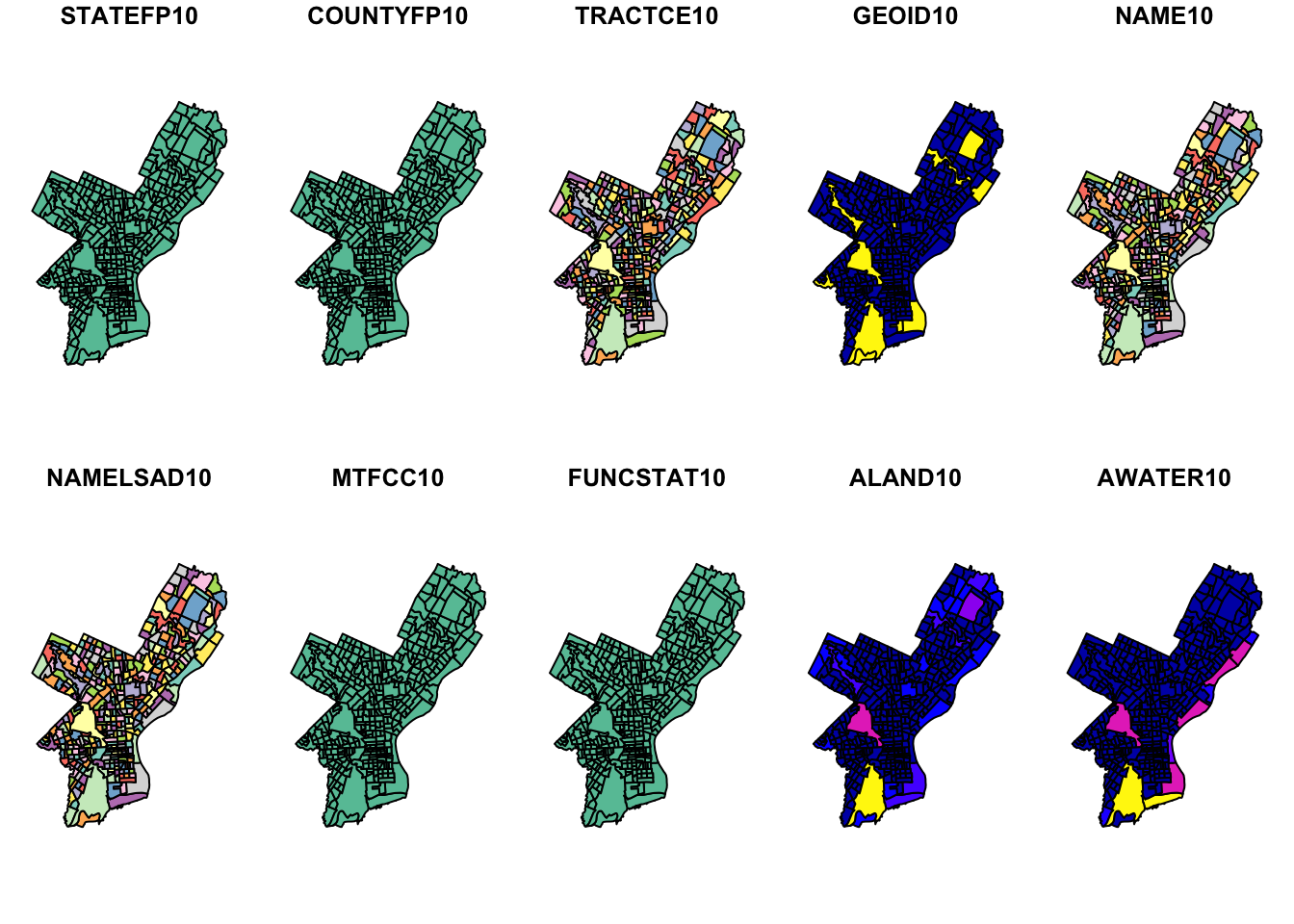
To make it a little cleaner, we can only plot the polygon boundariesn and forget about the attributes. For this we need to directly use the geometry column. We use the st_geometry() function again here, which extracts the sfc object (the simple feature geometry list column):

plot(st_geometry(philly_sf))

Alternatively, we can choose the attributes that we what to plot:

# plot - alternatives
plot(philly_sf["medHHinc"]) # subset with base R

philly_sf %>% select(medHHinc) %>%  plot() # piping with tidyverse

Now let’s get a little fancier.

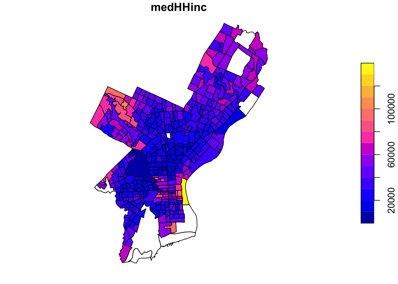
Let’s add a subset of polygons with only the census tracts where the median houshold income (medHHinc) is more than $60,000. First we plot the polygon. Then in a second step we extract elements from an sf object based on attributes using the dplyr filter function (base R subsetting also works) and add the census tracts to the plot in a different color.

# step 1 - plot empty polylgons:
plot(st_geometry(philly_sf)) 

# step 2 - add colored polygons on top
philly_sf %>% 
  filter(medHHinc > 60000) %>% # filter for high income
  st_geometry() %>% # extract the geometry for plotting
  plot(col="red", add=T) # add to the plot

1.4 Raster data in R

Raster files, as you might know, have a more compact data structure than vectors. Because of their regular structure the coordinates do not need to be recorded for each pixel or cell in the rectangular extent. A raster is defined by:

  • a CRS
  • coordinates of its origin
  • a distance or cell size in each direction
  • a dimension or numbers of cells in each direction
  • an array of cell values

Given this structure, coordinates for any cell can be computed and don’t need to be stored.

terra was first released in 2020 and now replaces the raster package which was first released in 2010. terra has greater functionality, is faster and easier to use.

raster vs terra downloads on CRAN

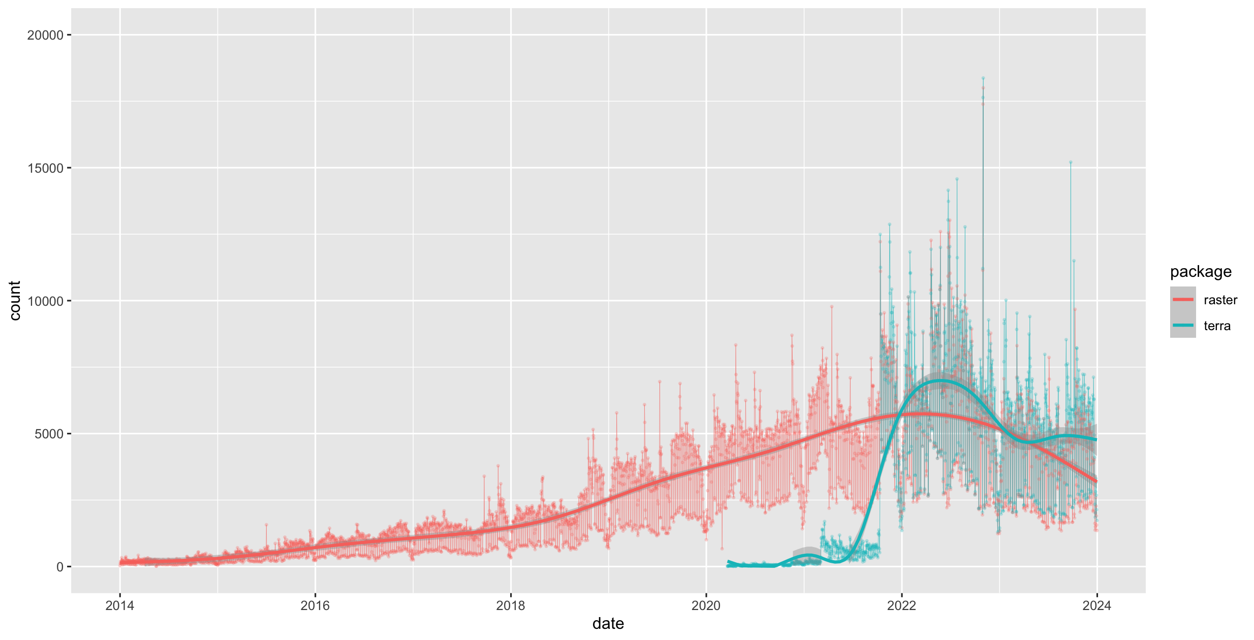
Figure 1.4: raster vs terra downloads on CRAN

The terra package has functions for creating, reading, manipulating, and writing raster data. The package also implements raster algebra and many other functions for raster data manipulation.

The package works with SpatRaster objects. The rast() function is used to create these objects. For example, to create a raster object from scratch we would do the following:

library(terra)
r <- rast(nrows=20, ncols=20, # number of cells in x and y dimension
          xmin=0, xmax=360) # min and max x coordinates (left-right borders)
r
#> class       : SpatRaster 
#> size        : 20, 20, 1  (nrow, ncol, nlyr)
#> resolution  : 18, 9  (x, y)
#> extent      : 0, 360, -90, 90  (xmin, xmax, ymin, ymax)
#> coord. ref. : lon/lat WGS 84 (CRS84) (OGC:CRS84)

From the output above we know that:

  • the object is of class SpatRaster
  • its dimensions are 20x20 cells
  • it has one layer (band)
  • the extent of the raster
  • it has a CRS defined! If the crs argument is missing when creating the SpatRaster object, if the x coordinates are within -360 and 360 and the y coordinates are within -90 and 90, the WGS84 projection is used by default.

Good to know.

There are functions to look at individual properties of the raster object. For examle for the number of cells:

ncell(r)
#> [1] 400

Or we can retrieve just the number of bands using the nlyr() function.

nlyr(r)
#> [1] 1

We can also find out about the Coordinate Reference System (CRS) with the crs function. The default output looks a little messy:

crs(r)
#> [1] "GEOGCRS[\"WGS 84 (CRS84)\",\n    DATUM[\"World Geodetic System 1984\",\n        ELLIPSOID[\"WGS 84\",6378137,298.257223563,\n            LENGTHUNIT[\"metre\",1]]],\n    PRIMEM[\"Greenwich\",0,\n        ANGLEUNIT[\"degree\",0.0174532925199433]],\n    CS[ellipsoidal,2],\n        AXIS[\"geodetic longitude (Lon)\",east,\n            ORDER[1],\n            ANGLEUNIT[\"degree\",0.0174532925199433]],\n        AXIS[\"geodetic latitude (Lat)\",north,\n            ORDER[2],\n            ANGLEUNIT[\"degree\",0.0174532925199433]],\n    USAGE[\n        SCOPE[\"unknown\"],\n        AREA[\"World\"],\n        BBOX[-90,-180,90,180]],\n    ID[\"OGC\",\"CRS84\"]]"

We can make this easier to read by setting the proj argument:

crs(r, proj = TRUE) # return the PROJ-string notation
#> [1] "+proj=longlat +datum=WGS84 +no_defs"

Let’s try and plot this.

plot(r)

The canvas is empty! This is because even though we have a layer, the cells do not have any values.

values(r)

To add some random values to the cells we can take advantage of the ncells() function and do this:

values(r) <- runif(ncell(r))
r 
#> class       : SpatRaster 
#> size        : 20, 20, 1  (nrow, ncol, nlyr)
#> resolution  : 18, 9  (x, y)
#> extent      : 0, 360, -90, 90  (xmin, xmax, ymin, ymax)
#> coord. ref. : lon/lat WGS 84 (CRS84) (OGC:CRS84) 
#> source(s)   : memory
#> name        :        lyr.1 
#> min value   : 0.0002538064 
#> max value   : 0.9989342857

In addition to the output above, we now see:

  • the source, which indicates where the cell values are stored (here they are in memory)
  • the range of the cell values (min value adn max value) now added.
  • the name, of the layer which is by default lyr.1.

This now plots successfully:

plot(r)

(The rasterVis package provides a set of methods for enhanced visualization and interaction for more advanced plotting of raster objects.)

SpatRaster objects can also be created from a matrix.

class(volcano)
#> [1] "matrix" "array"
volcano.r <- rast(volcano)
class(volcano.r)
#> [1] "SpatRaster"
#> attr(,"package")
#> [1] "terra"

We also use the rast() function to read in a raster file. This raster is generated as part of the NEON Harvard Forest field site.

HARV <- rast("data/HARV_RGB_Ortho.tif")

Typing the name of the object will give us what’s in there:

HARV
#> class       : SpatRaster 
#> size        : 2317, 3073, 3  (nrow, ncol, nlyr)
#> resolution  : 0.25, 0.25  (x, y)
#> extent      : 731998.5, 732766.8, 4712956, 4713536  (xmin, xmax, ymin, ymax)
#> coord. ref. : WGS 84 / UTM zone 18N (EPSG:32618) 
#> source      : HARV_RGB_Ortho.tif 
#> names       : HARV_RGB_Ortho_1, HARV_RGB_Ortho_2, HARV_RGB_Ortho_3 
#> min values  :                0,                0,                0 
#> max values  :              255,              255,              255

Challenge

Based on the output above answer the following questions:

  1. How many bands?
  2. What are the names of the bands)?
  3. Where on the system are the cell values stored?
  4. What is the CRS?

We can plot the object like this:

plot(HARV)

Or to plot a single band:

plot(HARV, 3)

We can also use the rast() function to import one single band:

HARV_Band2 <- rast("data/HARV_RGB_Ortho.tif", lyrs = 2)
plot(HARV_Band2)

Let’s now explore the distribution of values contained within our raster using the hist() function which produces a histogram. Histograms are often useful in identifying outliers and bad data values in our raster data.

hist(HARV)
#> Warning: [hist] a sample of 14% of the cells was used

Notice that a warning message is produced when R creates the histogram. By default the maximum cells processed per band is 1,000,000. This maximum value is to ensure processing efficiency as our data become larger. We can force the hist function to use all cell values.

ncell(HARV)
#> [1] 7120141
hist(HARV, maxcell = ncell(HARV))

At times it may be useful to explore raster metadata before loading them into R. This can be done with the function describe()

describe("data/HARV_RGB_Ortho.tif")
#>  [1] "Driver: GTiff/GeoTIFF"                                                                                                                                                                                                                                                          
#>  [2] "Files: data/HARV_RGB_Ortho.tif"                                                                                                                                                                                                                                                 
#>  [3] "Size is 3073, 2317"                                                                                                                                                                                                                                                             
#>  [4] "Coordinate System is:"                                                                                                                                                                                                                                                          
#>  [5] "PROJCRS[\"WGS 84 / UTM zone 18N\","                                                                                                                                                                                                                                             
#>  [6] "    BASEGEOGCRS[\"WGS 84\","                                                                                                                                                                                                                                                    
#>  [7] "        ENSEMBLE[\"World Geodetic System 1984 ensemble\","                                                                                                                                                                                                                      
#>  [8] "            MEMBER[\"World Geodetic System 1984 (Transit)\"],"                                                                                                                                                                                                                  
#>  [9] "            MEMBER[\"World Geodetic System 1984 (G730)\"],"                                                                                                                                                                                                                     
#> [10] "            MEMBER[\"World Geodetic System 1984 (G873)\"],"                                                                                                                                                                                                                     
#> [11] "            MEMBER[\"World Geodetic System 1984 (G1150)\"],"                                                                                                                                                                                                                    
#> [12] "            MEMBER[\"World Geodetic System 1984 (G1674)\"],"                                                                                                                                                                                                                    
#> [13] "            MEMBER[\"World Geodetic System 1984 (G1762)\"],"                                                                                                                                                                                                                    
#> [14] "            MEMBER[\"World Geodetic System 1984 (G2139)\"],"                                                                                                                                                                                                                    
#> [15] "            MEMBER[\"World Geodetic System 1984 (G2296)\"],"                                                                                                                                                                                                                    
#> [16] "            ELLIPSOID[\"WGS 84\",6378137,298.257223563,"                                                                                                                                                                                                                        
#> [17] "                LENGTHUNIT[\"metre\",1]],"                                                                                                                                                                                                                                      
#> [18] "            ENSEMBLEACCURACY[2.0]],"                                                                                                                                                                                                                                            
#> [19] "        PRIMEM[\"Greenwich\",0,"                                                                                                                                                                                                                                                
#> [20] "            ANGLEUNIT[\"degree\",0.0174532925199433]],"                                                                                                                                                                                                                         
#> [21] "        ID[\"EPSG\",4326]],"                                                                                                                                                                                                                                                    
#> [22] "    CONVERSION[\"UTM zone 18N\","                                                                                                                                                                                                                                               
#> [23] "        METHOD[\"Transverse Mercator\","                                                                                                                                                                                                                                        
#> [24] "            ID[\"EPSG\",9807]],"                                                                                                                                                                                                                                                
#> [25] "        PARAMETER[\"Latitude of natural origin\",0,"                                                                                                                                                                                                                            
#> [26] "            ANGLEUNIT[\"degree\",0.0174532925199433],"                                                                                                                                                                                                                          
#> [27] "            ID[\"EPSG\",8801]],"                                                                                                                                                                                                                                                
#> [28] "        PARAMETER[\"Longitude of natural origin\",-75,"                                                                                                                                                                                                                         
#> [29] "            ANGLEUNIT[\"degree\",0.0174532925199433],"                                                                                                                                                                                                                          
#> [30] "            ID[\"EPSG\",8802]],"                                                                                                                                                                                                                                                
#> [31] "        PARAMETER[\"Scale factor at natural origin\",0.9996,"                                                                                                                                                                                                                   
#> [32] "            SCALEUNIT[\"unity\",1],"                                                                                                                                                                                                                                            
#> [33] "            ID[\"EPSG\",8805]],"                                                                                                                                                                                                                                                
#> [34] "        PARAMETER[\"False easting\",500000,"                                                                                                                                                                                                                                    
#> [35] "            LENGTHUNIT[\"metre\",1],"                                                                                                                                                                                                                                           
#> [36] "            ID[\"EPSG\",8806]],"                                                                                                                                                                                                                                                
#> [37] "        PARAMETER[\"False northing\",0,"                                                                                                                                                                                                                                        
#> [38] "            LENGTHUNIT[\"metre\",1],"                                                                                                                                                                                                                                           
#> [39] "            ID[\"EPSG\",8807]]],"                                                                                                                                                                                                                                               
#> [40] "    CS[Cartesian,2],"                                                                                                                                                                                                                                                           
#> [41] "        AXIS[\"(E)\",east,"                                                                                                                                                                                                                                                     
#> [42] "            ORDER[1],"                                                                                                                                                                                                                                                          
#> [43] "            LENGTHUNIT[\"metre\",1]],"                                                                                                                                                                                                                                          
#> [44] "        AXIS[\"(N)\",north,"                                                                                                                                                                                                                                                    
#> [45] "            ORDER[2],"                                                                                                                                                                                                                                                          
#> [46] "            LENGTHUNIT[\"metre\",1]],"                                                                                                                                                                                                                                          
#> [47] "    USAGE["                                                                                                                                                                                                                                                                     
#> [48] "        SCOPE[\"Navigation and medium accuracy spatial referencing.\"],"                                                                                                                                                                                                        
#> [49] "        AREA[\"Between 78°W and 72°W, northern hemisphere between equator and 84°N, onshore and offshore. Bahamas. Canada - Nunavut; Ontario; Quebec. Colombia. Cuba. Ecuador. Greenland. Haiti. Jamaica. Panama. Turks and Caicos Islands. United States (USA). Venezuela.\"],"
#> [50] "        BBOX[0,-78,84,-72]],"                                                                                                                                                                                                                                                   
#> [51] "    ID[\"EPSG\",32618]]"                                                                                                                                                                                                                                                        
#> [52] "Data axis to CRS axis mapping: 1,2"                                                                                                                                                                                                                                             
#> [53] "Origin = (731998.500000000000000,4713535.500000000000000)"                                                                                                                                                                                                                      
#> [54] "Pixel Size = (0.250000000000000,-0.250000000000000)"                                                                                                                                                                                                                            
#> [55] "Metadata:"                                                                                                                                                                                                                                                                      
#> [56] "  AREA_OR_POINT=Area"                                                                                                                                                                                                                                                           
#> [57] "Image Structure Metadata:"                                                                                                                                                                                                                                                      
#> [58] "  COMPRESSION=LZW"                                                                                                                                                                                                                                                              
#> [59] "  INTERLEAVE=PIXEL"                                                                                                                                                                                                                                                             
#> [60] "Corner Coordinates:"                                                                                                                                                                                                                                                            
#> [61] "Upper Left  (  731998.500, 4713535.500) ( 72d10'29.27\"W, 42d32'21.80\"N)"                                                                                                                                                                                                      
#> [62] "Lower Left  (  731998.500, 4712956.250) ( 72d10'30.11\"W, 42d32' 3.04\"N)"                                                                                                                                                                                                      
#> [63] "Upper Right (  732766.750, 4713535.500) ( 72d 9'55.63\"W, 42d32'20.97\"N)"                                                                                                                                                                                                      
#> [64] "Lower Right (  732766.750, 4712956.250) ( 72d 9'56.48\"W, 42d32' 2.21\"N)"                                                                                                                                                                                                      
#> [65] "Center      (  732382.625, 4713245.875) ( 72d10'12.87\"W, 42d32'12.00\"N)"                                                                                                                                                                                                      
#> [66] "Band 1 Block=3073x1 Type=Float64, ColorInterp=Gray"                                                                                                                                                                                                                             
#> [67] "  Min=0.000 Max=255.000 "                                                                                                                                                                                                                                                       
#> [68] "  Minimum=0.000, Maximum=255.000, Mean=nan, StdDev=nan"                                                                                                                                                                                                                         
#> [69] "  NoData Value=-1.7e+308"                                                                                                                                                                                                                                                       
#> [70] "  Metadata:"                                                                                                                                                                                                                                                                    
#> [71] "    STATISTICS_MAXIMUM=255"                                                                                                                                                                                                                                                     
#> [72] "    STATISTICS_MEAN=nan"                                                                                                                                                                                                                                                        
#> [73] "    STATISTICS_MINIMUM=0"                                                                                                                                                                                                                                                       
#> [74] "    STATISTICS_STDDEV=nan"                                                                                                                                                                                                                                                      
#> [75] "Band 2 Block=3073x1 Type=Float64, ColorInterp=Undefined"                                                                                                                                                                                                                        
#> [76] "  Min=0.000 Max=255.000 "                                                                                                                                                                                                                                                       
#> [77] "  Minimum=0.000, Maximum=255.000, Mean=nan, StdDev=nan"                                                                                                                                                                                                                         
#> [78] "  NoData Value=-1.7e+308"                                                                                                                                                                                                                                                       
#> [79] "  Metadata:"                                                                                                                                                                                                                                                                    
#> [80] "    STATISTICS_MAXIMUM=255"                                                                                                                                                                                                                                                     
#> [81] "    STATISTICS_MEAN=nan"                                                                                                                                                                                                                                                        
#> [82] "    STATISTICS_MINIMUM=0"                                                                                                                                                                                                                                                       
#> [83] "    STATISTICS_STDDEV=nan"                                                                                                                                                                                                                                                      
#> [84] "Band 3 Block=3073x1 Type=Float64, ColorInterp=Undefined"                                                                                                                                                                                                                        
#> [85] "  Min=0.000 Max=255.000 "                                                                                                                                                                                                                                                       
#> [86] "  Minimum=0.000, Maximum=255.000, Mean=nan, StdDev=nan"                                                                                                                                                                                                                         
#> [87] "  NoData Value=-1.7e+308"                                                                                                                                                                                                                                                       
#> [88] "  Metadata:"                                                                                                                                                                                                                                                                    
#> [89] "    STATISTICS_MAXIMUM=255"                                                                                                                                                                                                                                                     
#> [90] "    STATISTICS_MEAN=nan"                                                                                                                                                                                                                                                        
#> [91] "    STATISTICS_MINIMUM=0"                                                                                                                                                                                                                                                       
#> [92] "    STATISTICS_STDDEV=nan"

For the many functions available for working with such an object see:

methods(class="SpatRaster")
#>   [1] !                     [                     [[                   
#>   [4] [[<-                  [<-                   %in%                 
#>   [7] $                     $<-                   activeCat            
#>  [10] activeCat<-           add<-                 addCats              
#>  [13] adjacent              aggregate             align                
#>  [16] all.equal             allNA                 animate              
#>  [19] anyNA                 app                   approximate          
#>  [22] area                  Arith                 as.array             
#>  [25] as.bool               as.character          as.contour           
#>  [28] as.data.frame         as.factor             as.int               
#>  [31] as.integer            as.lines              as.list              
#>  [34] as.logical            as.matrix             as.numeric           
#>  [37] as.points             as.polygons           as.raster            
#>  [40] atan_2                atan2                 autocor              
#>  [43] barplot               bestMatch             blocks               
#>  [46] boundaries            boxplot               buffer               
#>  [49] c                     catalyze              categories           
#>  [52] cats                  cellFromRowCol        cellFromRowColCombine
#>  [55] cellFromXY            cells                 cellSize             
#>  [58] clamp_ts              clamp                 classify             
#>  [61] click                 coerce                colFromCell          
#>  [64] colFromX              colMeans              colorize             
#>  [67] colSums               coltab                coltab<-             
#>  [70] Compare               compare               compareGeom          
#>  [73] concats               contour               costDist             
#>  [76] countNA               cover                 crds                 
#>  [79] crop                  crosstab              crs                  
#>  [82] crs<-                 datatype              deepcopy             
#>  [85] density               depth                 depth<-              
#>  [88] depthName             depthName<-           depthUnit            
#>  [91] depthUnit<-           describe              diff                 
#>  [94] dim                   dim<-                 direction            
#>  [97] disagg                distance              divide               
#> [100] droplevels            expanse               ext                  
#> [103] ext<-                 extend                extract              
#> [106] extractRange          fillTime              flip                 
#> [109] flowAccumulation      focal                 focal3D              
#> [112] focalCpp              focalPairs            focalReg             
#> [115] focalValues           freq                  getTileExtents       
#> [118] global                gridDist              gridDistance         
#> [121] has.colors            has.RGB               has.time             
#> [124] hasMinMax             hasValues             head                 
#> [127] hist                  identical             ifel                 
#> [130] image                 init                  inMemory             
#> [133] inset                 interpIDW             interpNear           
#> [136] interpolate           intersect             is.bool              
#> [139] is.factor             is.finite             is.flipped           
#> [142] is.infinite           is.int                is.lonlat            
#> [145] is.na                 is.nan                is.num               
#> [148] is.related            is.rotated            isFALSE              
#> [151] isTRUE                k_means               lapp                 
#> [154] layerCor              levels                levels<-             
#> [157] linearUnits           lines                 log                  
#> [160] Logic                 logic                 longnames            
#> [163] longnames<-           makeTiles             mask                 
#> [166] match                 math                  Math                 
#> [169] Math2                 mean                  median               
#> [172] merge                 meta                  metags               
#> [175] metags<-              minmax                modal                
#> [178] mosaic                NAflag                NAflag<-             
#> [181] names                 names<-               ncell                
#> [184] ncol                  ncol<-                NIDP                 
#> [187] nlyr                  nlyr<-                noNA                 
#> [190] not.na                nrow                  nrow<-               
#> [193] nsrc                  origin                origin<-             
#> [196] pairs                 panel                 patches              
#> [199] persp                 pitfinder             plet                 
#> [202] plot                  plotRGB               points               
#> [205] polys                 prcomp                predict              
#> [208] princomp              project               quantile             
#> [211] rangeFill             rapp                  rast                 
#> [214] rasterize             rasterizeGeom         rasterizeWin         
#> [217] rcl                   readStart             readStop             
#> [220] readValues            rectify               regress              
#> [223] relate                rep                   res                  
#> [226] res<-                 resample              rescale              
#> [229] rev                   RGB                   RGB<-                
#> [232] roll                  rotate                rowColCombine        
#> [235] rowColFromCell        rowFromCell           rowFromY             
#> [238] rowMeans              rowSums               sapp                 
#> [241] saveRDS               scale_linear          scale                
#> [244] scoff                 scoff<-               sds                  
#> [247] segregate             sel                   selectHighest        
#> [250] selectRange           serialize             set.cats             
#> [253] set.crs               set.ext               set.names            
#> [256] set.RGB               set.values            set.window           
#> [259] setMinMax             setValues             shift                
#> [262] show                  sieve                 simplifyLevels       
#> [265] size                  sort                  sources              
#> [268] spatSample            split                 sprc                 
#> [271] st_bbox               st_crs                stdev                
#> [274] str                   stretch               subset               
#> [277] subst                 summary               Summary              
#> [280] surfArea              t                     tail                 
#> [283] tapp                  terrain               text                 
#> [286] thresh                tighten               time                 
#> [289] time<-                timeInfo              toMemory             
#> [292] trans                 trim                  unique               
#> [295] units                 units<-               update               
#> [298] values                values<-              varnames             
#> [301] varnames<-            viewshed              watershed            
#> [304] weighted.mean         where.max             where.min            
#> [307] which.lyr             which.max             which.min            
#> [310] window                window<-              wrap                 
#> [313] wrapCache             writeCDF              writeRaster          
#> [316] writeStart            writeStop             writeValues          
#> [319] xapp                  xFromCell             xFromCol             
#> [322] xmax                  xmax<-                xmin                 
#> [325] xmin<-                xres                  xyFromCell           
#> [328] yFromCell             yFromRow              ymax                 
#> [331] ymax<-                ymin                  ymin<-               
#> [334] yres                  zonal                 zoom                 
#> see '?methods' for accessing help and source code