Accessing World Bank Data from R
cengel @ stanford
Last updated: October 28, 2016
Background
From Shaefer et al 2016:
Can Poverty in America Be Compared to Conditions in the World’s Poorest Countries?
World Development Indicators used in this example:
- GDP per capita (constant 2010 US$)
- Life expectancy at birth, total (years)
- Mortality rate, infant (per 1,000 live births)
There are currently two R packages on CRAN with some differences, we compare them here:
1. Get data
First we download an updated list of inidicators. Both packages come with a downloaded list. That list appears to be still current for wbstats, as it is a newer package, for WDI however it is not up to date.
wbstats
library(wbstats)
new_wb_cache <- wbcache()
WDI
library(WDI)
new_wdi_cache <- WDIcache()
Next we find out the IDs for the indicators we are intersted in: GDP, life expectancy, and infant mortality.
Both packages support regular expressions for the search for indicator IDs.
wbstats
wbsearch("gdp.*capita.*US\\$", cache = new_wb_cache)## indicatorID indicator
## 7728 NY.GDP.PCAP.CD GDP per capita (current US$)
## 7730 NY.GDP.PCAP.KD GDP per capita (constant 2010 US$)wbsearch("life expectancy at birth.*total", cache = new_wb_cache)## indicatorID indicator
## 14389 SP.DYN.LE00.IN Life expectancy at birth, total (years)wbsearch("^mortality.*rate.*infant", cache = new_wb_cache)## indicatorID
## 14380 SP.DYN.IMRT.FE.IN
## 14381 SP.DYN.IMRT.IN
## 14382 SP.DYN.IMRT.MA.IN
## indicator
## 14380 Mortality rate, infant, female (per 1,000 live births)
## 14381 Mortality rate, infant (per 1,000 live births)
## 14382 Mortality rate, infant, male (per 1,000 live births)WDI
WDIsearch("gdp.*capita.*US\\$", cache = new_wdi_cache)## indicator name
## [1,] "NY.GDP.PCAP.CD" "GDP per capita (current US$)"
## [2,] "NY.GDP.PCAP.KD" "GDP per capita (constant 2010 US$)"WDIsearch("life expectancy at birth.*total", cache = new_wdi_cache)## indicator
## "SP.DYN.LE00.IN"
## name
## "Life expectancy at birth, total (years)"WDIsearch("^mortality.*rate.*infant", cache = new_wdi_cache)## indicator
## [1,] "SP.DYN.IMRT.FE.IN"
## [2,] "SP.DYN.IMRT.IN"
## [3,] "SP.DYN.IMRT.MA.IN"
## name
## [1,] "Mortality rate, infant, female (per 1,000 live births)"
## [2,] "Mortality rate, infant (per 1,000 live births)"
## [3,] "Mortality rate, infant, male (per 1,000 live births)"Finally we download the data. The download functions provided in the two packages mainly differ in their arguments and in the format of the data they return.
The WDI()function takes the argument extra=.. which can be set to TRUE to download more data fields (e.g. region, iso3c code, income_level).
The the wb() function does not have these particular options. In order to get this additional information (for exampe, to link countries to regions) it is necessary to download a separate table. Note, though that wb() comes with other options (e.g. download of quarterly or monthly data, most recent values) that WDI() does not have.
wbstats
wb_dat <- wb(indicator = c("NY.GDP.PCAP.KD", "SP.DYN.LE00.IN", "SP.DYN.IMRT.IN"))
names(wb_dat)
## [1] "value" "date" "indicatorID" "indicator" "iso2c"
## [6] "country"WDI
wdi_dat <- WDI(indicator = c("NY.GDP.PCAP.KD", "SP.DYN.LE00.IN", "SP.DYN.IMRT.IN"), start = 1960, end = 2015, extra = TRUE)
names(wdi_dat)
## [1] "iso2c" "country" "year" "NY.GDP.PCAP.KD"
## [5] "SP.DYN.LE00.IN" "SP.DYN.IMRT.IN" "iso3c" "region"
## [9] "capital" "longitude" "latitude" "income"
## [13] "lending"WDI() returns a data frame in wide format. Rows are per year and country/region, columns are the different indicators.
wb() returns a data frame in long format. Each row is one observation.
2. Clean up
We remove all entries that are aggregated regional values.
Using the wbstats package we need to add two extra steps to download a separate table with the regions names and join it to our data table before eliminating the undesired rows.
wbstats
wb_countries <- wbcountries()
names(wb_countries)
## [1] "iso3c" "iso2c" "country" "capital" "long"
## [6] "lat" "regionID" "region" "adminID" "admin"
## [11] "incomeID" "income" "lendingID" "lending"wb_dat <- merge(wb_dat, y = wb_countries[c("iso2c", "region")], by = "iso2c", all.x = TRUE)
wb_dat <- subset(wb_dat, region != "Aggregates") # this also removes NAsWDI
wdi_dat <- subset(wdi_dat, region != "Aggregates") # this also removes NAsNow we rename the indicators to something we understand better.
With wbstats we need to add an extra step to reformat the table into wide format that we will use as input for the plotting.
wbstats
wb_dat$indicatorID[wb_dat$indicatorID == "NY.GDP.PCAP.KD"] <- "GDP"
wb_dat$indicatorID[wb_dat$indicatorID == "SP.DYN.LE00.IN"] <- "life_expectancy"
wb_dat$indicatorID[wb_dat$indicatorID == "SP.DYN.IMRT.IN"] <- "infant_mortality"

library(reshape2)
wb_dat <- dcast(wb_dat, iso2c + country + date + region ~ indicatorID,  value.var = 'value')
WDI
names(wdi_dat)[which(names(wdi_dat) == "NY.GDP.PCAP.KD")] <- "GDP"
names(wdi_dat)[which(names(wdi_dat) == "SP.DYN.LE00.IN")] <- "life_expectancy"
names(wdi_dat)[which(names(wdi_dat) == "SP.DYN.IMRT.IN")] <- "infant_mortality"
Now we have pretty much identical tables.
3. Plot a graph
wbstats
library(ggplot2)
ggplot(subset(wb_dat, date == "2008"), aes(x = GDP, y = infant_mortality)) + geom_point()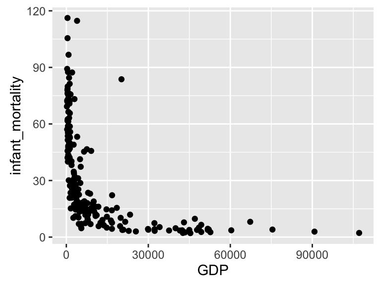
WDI
ggplot(subset(wdi_dat, year == 2008), aes(x = GDP, y = infant_mortality)) + geom_point()
4. Reproduce graphs from the paper
Life Expectancy
lifexp_countries <- subset(wb_dat, country %in% c("United States", "Rwanda", "Mongolia", "Pakistan", "Lao PDR", "Bhutan", "Malaysia", "Brazil", "Ireland", "Japan", "Sweden", "Netherlands"))

ggplot(subset(lifexp_countries, date == "2008"), aes(x = GDP, y = life_expectancy, color = country == "United States")) +
  geom_point() +
  geom_text(aes(label = country), size=3, nudge_y = 0.4) +
  scale_x_continuous(limits = c(0, 70000))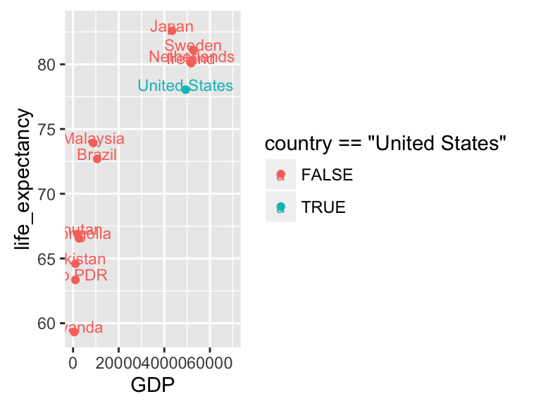
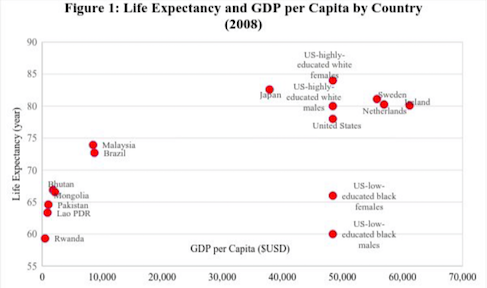
(From Shaefer et al 2016)
Infant Mortality
infmort_countries <- subset(wb_dat, country %in% c("United States", "Tonga", "Colombia", "Grenada", "Sri Lanka", "Malta", "Germany", "Japan", "Sweden", "Netherlands"))

ggplot(subset(infmort_countries, date == "2008"), aes(x = GDP, y = infant_mortality, color = country == "United States")) +
  geom_point() +
  geom_text(aes(label = country), size=3, nudge_y = 0.2) +
  scale_x_continuous(limits = c(0, 70000))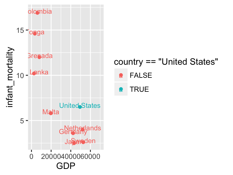
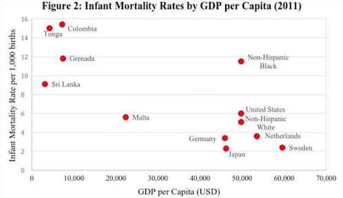
(From Shaefer et al 2016)
5. Simple interactivity
library(plotly)

g <- ggplot(subset(infmort_countries, date > "1999" & date <= "2015"), aes(x = GDP, y = infant_mortality, color = country == "United States", tooltip = country)) +
  geom_point() +
  facet_wrap(~ date) +
  theme(legend.position="none")

ggplotly(g)
Reference:
H. Luke Shaefer, Pinghui Wu, Kathryn Edin, 2016: Can Poverty in America Be Compared to Conditions in the World’s Poorest Countries? Publication, Stanford Center on Poverty & Inequality. http://inequality.stanford.edu/publications/media/details/can-poverty-america-be-compared-conditions-worlds-poorest-countries